Algorithm Update

As discussed, we think it might be a good idea to stop the fitting in an algorithmic way. As we noticed, as we go deeper and deeper the ratio of failed fits to successful fits increases. I haven’t implemented this in the code (yet), but it is something to come back to if we decide this is a good way to go.

• One we have all our successful fits, we sort them based on some parameter specified by the user (default would be magnitude or surface brightness)
• As we fit, we store the previous, say, 50 results (successful or failure) in an array.
• After 50 fits, we start to check the ratio of successes to failures.
• If the ratio slips too much into being failure dominated, (say, 50 or 60%), we stop the fitting.

This would be a good automated way to stop the fitting once too many failures are occurring.

ACEnet Meeting Planned!

During this week, I spent some time moving some of my work onto the Cedar cluster. For whatever reason, the bash script that I used on my previous pipeline is no longer valid for my new pipeline. This means it was definitely time to schedule a meeting with a rep from ACEnet.
On Wednesday afternoon next week, I will meet with Ross Dickson (who I have already met from the parallel computing school!). The things I will go over are as follows:

• How do I properly get Astropy, Photutils, and other Conda packages setup, and do I have to run this setup for every job?
• How can I handle fail conditions (such as the dreaded infinite loop issue). Something I might do is have an internal timer running on a different thread, and any last-minute commands (such as image deletion) will always be run if this timer is triggered in the final few minutes just in case.
• Is the area in which I am doing parallelization (at the individual image level) a good place to do it? Would it be better to parallelize things at the individual object level?

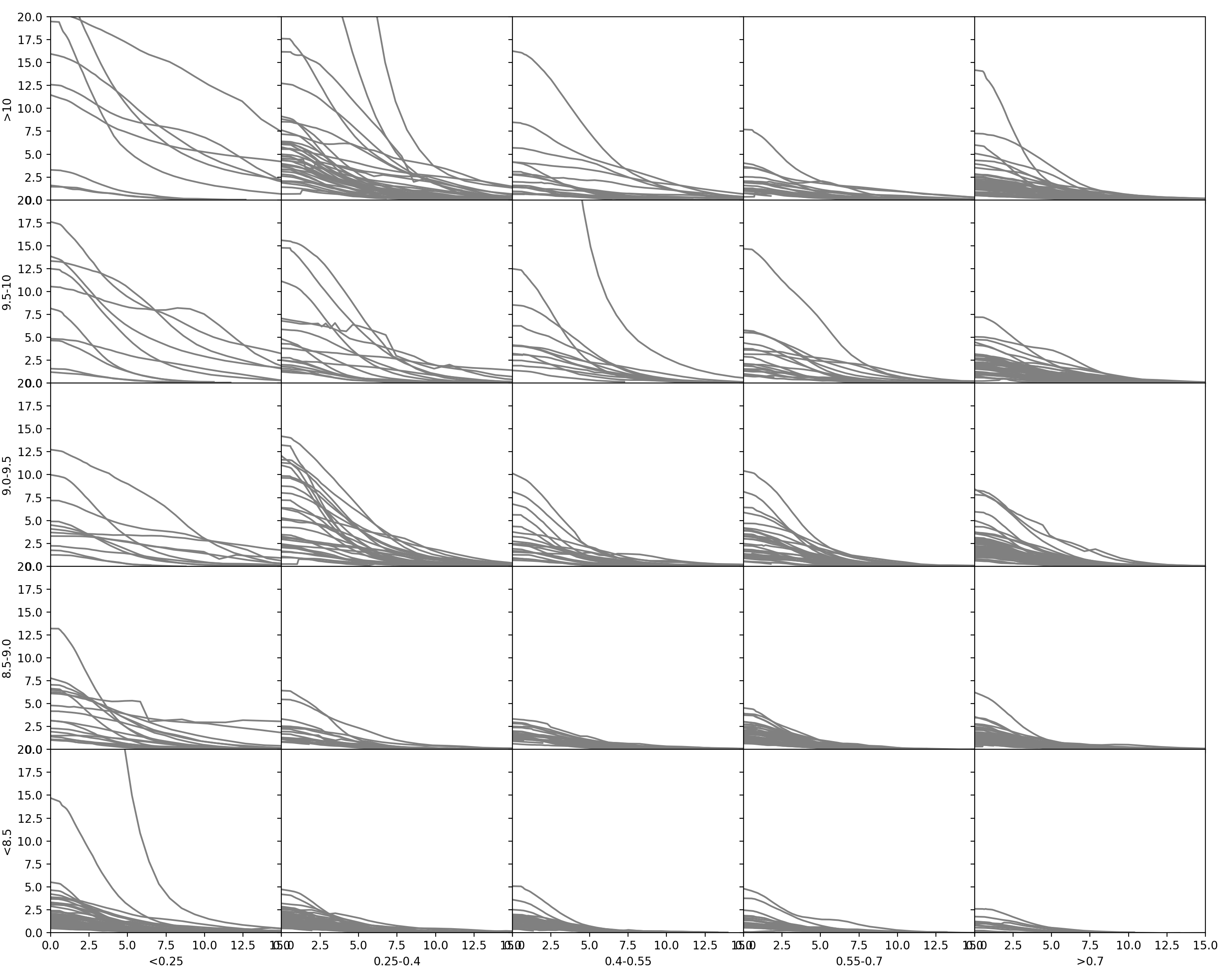
Multiband Histograms

As discussed, we want to see what our cutoffs might be across different bands. Thus, I have prepared the same scatter plots for every band. I attempted to fit 500 objects in all 7 images (G, R, I, Z, Y, U, U*) and have included the results. All the figures (including scatter plots) are included in the Dropbox under Figures/Multiband Testing if you would like to explore things further. To keep things simple, I have only posted the stacked magnitude and surface brightness histograms.

Surface Brightness Histograms

• 

• 

• 

• 

• 

• 

• 

Magnitude Histograms

• 

• 

• 

• 

• 

• 

• 

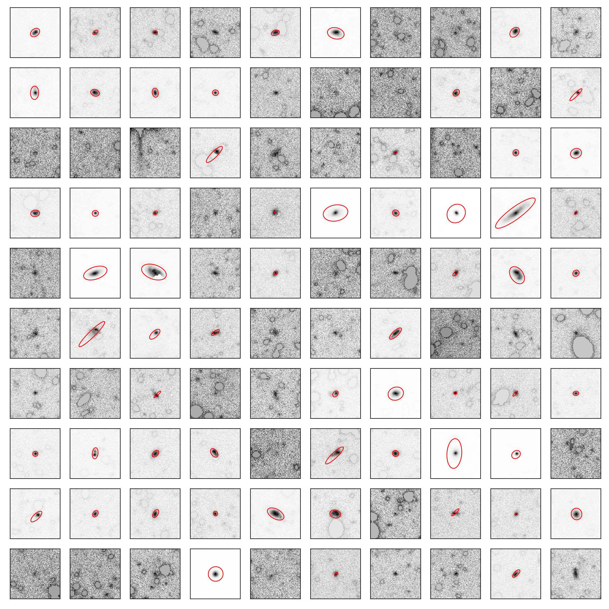
Matrix Plot Revamp

I realized early on that there is some motivation to rewrite the matrix plot code. The code, in similar fashion to the old pipeline, is very difficult to adjust or set up to work with the newly generated data.
I am currently rewriting the matrix plot code to better accommodate easier adjustments. It is now very easy to change the values for binning, or even the number of bins that exist. Below is the current iteration of the matrix plot, binned by mass on the Y-axis and Redshift on the X-axis. By tomorrow, there will be medians added to these plots.

Final Addendum

Moving forward, I have adjusted the catalogue to not have any cuts in either redshift or I-Band magnitude. These figures are not with this adjusted catalogue, but it shouldn’t make a hugely noticeable difference on what we see.

Where are things Failing?

To test which objects are failing to be fit, I attempted to fit 1000 objects in the 9813-4,3 patch in the u* band. I added to the pipeline another flag, -i, which will save the successful and failed IDs to two seperate files. I also remade the catalogue to contain the max Surface Brightness values for each unique band.

Below are a few plots for you to consider. You can click on them to view these figures in greater detail. Anything in red denotes an unsuccessful fit, and anything in green a successful fit. The first two are scatter plots comparing the I-Band Magnitude to u* Surface brightness and redshift. The remaining three are histograms of those three parameters. Just to clarify, the successful and unsuccessful bins are not stacked on top of each other.

• 

• 

• 

• 

• 

• 

This does seem to confirm my suspicion that the likelihood of success is strongly determined by magnitude. Surface Brightness seems to be an even better marker of when things fail. Looking at the i_mag vs u* SB scatter plot, we can see that the overwhelming majority of failed fits are above SB=26. I would have to guess that the few failures located in the brighter SB region are those “cigar shaped” galaxies that Ivana observed to be a second group in the failed cutouts.

Ellipticities at HLR and Maximum Ellipticity

Below are two histograms showing the distributions of ellipticities for two different places. At the ellipse with the maximum ellipticity, and at an estimation of the half-light radius.

• 

• 

U* Band Histograms and Scatter Plots

Below are figures identical to above, but instead of I-Band magnitude we plot U*-Band magnitude. Especially in the u* mag vs u* SB plot, we see a much clearer relation and the transition from predominantly successful to failure is clear. It also looks like the failed objects are “pushed up” more in the u* vs z plot.

• 

• 

• 

M* vs Z

Lots of interesting things to discuss about this week!

Koe Pipeline and Saving Outputs

The reworked pipeline, from input to output, is complete! All that remains is further experimentation in improving the fitting. I have added 3 methods to save output information:

1. The first is simply to save all the tables to one HDUList with no cutouts.
2. The second is to save two HDULists, one with the tables and another containing the cutouts. These could then be ID matched if required.
3. The third option is to save them the same way as last summer, with each profile and cutout having it’s own unique FITS file. While this method was fine last year, having such a larger dataset will make this method cumbersome.

One major takeaway from the ACEnet workshop was not to save many thousands of small files to a directory, so I think saving everything together in one large file is the best way to go. If we really want to have the cutouts, the option is still there.

I have also gotten parallelization to work! If processing a batch of images, you can have the pipeline process multiple images across different cores. This cuts the computation time down dramatically! We can start running jobs on ACEnet once we are happy with the fitting results.

Outside of work, I have also started an Overleaf project that outlines how the pipeline operates. It can be found at this link: https://www.overleaf.com/read/xsdsfgxprzbv. If you would like to have edit permissions, just let me know!

Success Rates in Different I-Band Magnitudes

Below is a figure showing the success rate of fits in different I-Band magnitude regions. I tested 100 cutouts in each band for each magnitude range, in steps of 0.5 from 21 to 25. The markers at 23.25 represent the region of 23-23.5, and so on. The thick black line represents the median value at each magnitude range. As expected, we see a pretty consistent downward trend.

Improving Fitting Results

As we discussed on Tuesday, using SExtractor morphological results so we have an initial guess would be a good means to possibly improve the code success rate. As it turns out, the photutils package photutils.morphology has a method that obtains the same information as SExtractor. According to the documentation, this package can do a better job than SExtractor. This is because, allegedly, SExtractor’s results will be done on a filtered image and return a less elliptical aperture than desired.

https://photutils.readthedocs.io/en/stable/morphology.html

https://photutils.readthedocs.io/en/stable/api/photutils.segmentation.SourceProperties.html#photutils.segmentation.SourceProperties

The apertures you see below are created based on the morphological results of fitting to the log of the data, versus the raw data. After doing some testing (including testing to fit apertures to the unaltered and square root of the data), I find this returns the most faithful apertures, and for the most objects. For very dim objects, you can see the source detection failing (no aperture shown) similar to what we saw in the Elliptical Isophote Fitting results.

I will change my fitting procedure to consider the ellipse generated by photutils.morphology as its initial guess. If this fails, I will go through my parameter space of initial ellipses as before. Thus, we should expect to only increase the success rate. How much of an increase I still have to explore, but I would be surprised if it was negligible.

The past week was very eventful, and I am happy with the progress made this week.

The Catalogue

To make processing the large catalogue easier, I made some cuts. The selections I made using TOPCAT are as follows:

1. Take only relevant columns from the catalogue. Instead of 177 columns, I am only taking ~50 that are relevant to my work.
2. Select all objects with CLASS=0 (Select only galaxies)
3. Select all objects with z < 0.9, and M* > 10 (Mass and redshift cuts)

This cuts the catalogue down to 210962 objects, and only 50 MB. Much easier to work with!

The Pipeline

Concerning the pipeline, I have two major updates.

The first is that I have completely overhauled the pipeline’s inner code, using Jupyter to test every step module by module. This is to improve efficiency and to ensure that everything is being done properly.

The second update, and the one I’m most excited about, is that I have configured the pipeline to run purely through the command line, taking the catalogue and image(s) as an argument. Not only will this make running things through ACEnet easier, but it will improve ease-of-use for anyone wanting to use the pipeline in the future.

I am also able to download URLs for the images using the code Ivana sent. I had to adjust the box search in the SQL lookup to include the COSMOS data, where I got the positional information visually from the figure below, (taken from the HSC DR2 Paper). The tract IDs appear to coincide with the ones in COSMOS, so I am confident I have the right information.

Ikuru’s code to print the URLs also required some adjusting. I will speak with you in our meeting to ensure that the output is correct, but opening one of the images (obtained using wget) in ds9 leads me to believe they are what we want.
NOTE: There is an issue present with the WCS that I am trying to obtain from the images. Whether I am simply looking at the wrong part of the datacube or the WCS is improperly formatted I am not sure. Without WCS, I cannot use RA and DEC to obtain cutouts. This is only an issue for the I-Band image, not the U-Band image.
There was also a bug in Ikuru’s code to take the image band as an extra argument, which I fixed. You can now specify which band you would like as a second argument. I’d like to send him the fixed version of the code, if you think it is worth sending!

I ran the updated pipeline on the U band image for 9813-4,3. This patch contained 487 objects, and the total fitting time was ~8 minutes. By adjusting the initial geometries that I attempt to fit, I was able to improve the percentage of objects successfully fit from 34% to 61% which is the current success rate. Obviously with numbers like that, it is worth checking to see why so many are failing. Below are two sets of cutouts. The first contains successful fits, the second unsuccessful. Just by observing the cutouts, it is clear that many of those failing tend to have a low signal-to-noise ratio. Perhaps a magnitude cut would also be something to consider?

WCS Issue – Addendum

I decided to check whether or not there was an issue with the WCS by opening up I-Band images (I downloaded another patch from the I-Band to ensure it wasn’t specific to one image), and comparing it to U-Band. I also checked to see if there were any other WCS headers in the image by checking row by row in the FITS HDUList, and as expected, there is only the one.

As you can see, the I-Band images are missing actual values in their WCS header data. This explains why my code wasn’t able to retrieve anything from them. Could it be that the images I am obtaining aren’t the ones we need?
An example URL is as follows:
https://hsc-release.mtk.nao.ac.jp/archive/filetree/pdr2_dud/deepCoadd/HSC-I/9813/3,4.fits

I do think I have a workaround however, referring back to Marcin’s idea of using the positional information from U-Band to make cutouts for the other bands. This would be very difficult to do at the base-code level, but I CAN adjust the WCS for the images once I have them all via WGET.
The procedure would be that I download all the images, get the WCS from the U-Band image and apply it to the other images. Any discrepancies would be equivalent to using the positions from the U-Band image, since I am still using the U-Band image’s WCS to determine where objects are.

Full Project Workflow

This diagram is to show how the entire project is structured, as well as how the outputs will be saved. We will have to have a discussion about how we want to save things. If we don’t want to keep the cutouts, we can save the output for an entire image as 1 FITS file, where each row is a table containing all the relevant data. However, keeping the cutouts poses a more difficult problem, and because of this last summer I saved each image as a separate file. Since we dealing with a far larger data sample, I will consider changing this.

Sersic Fitting – Next Steps

In our last meeting, Ivana and I talked about the current results of fitting Sersic profiles to our galaxies. These profiles are obtained by taking radial profiles from both our cutouts, and our models, to ensure the same extraction method is used. The figures compare the values from the SDSS catalogue to computed values, and all SDSS galaxies in that catalogue are represented here. As can be seen, the fitter is doing a decent job of fitting the effective radii, but a much worse job at obtaining a matching Sersic index.

One further step involves testing whether normalizing the radial profile to the profile obtained by Ellipse would retrieve a better value for the Sersic index. Following that, it would be a matter of testing more model galaxies and ensuring that the right values are being extracted, before moving forward with the full sample.

Since we are (hopefully) on the home stretch for this project, I am looking at the different methods of extracting a 1D profile from our 2D convolved image, and how those methods effect our final output parameters.

As I showed to Ivana yesterday, we are finding that using certain methods appear to return satisfactory values (larger Sersic indices for the SDSS galaxies), but the actual fit of the data isn’t very accurate. We have also seen the opposite when taking a slice through the 2D image to retrieve a profile, where the fit appears very good, but the values seem far too small. We can see these effects by observing the fits directly, and comparing the catalogue and computed values.

One interesting idea that Ivana suggested yesterday was for me to fit the observed galaxies with the radial profile method, and observe their differences. Below are a few results of that test.

Here’s the blue profile is the profile we calculated using ellipse(), and the orange profile is calculated using a simple radial profile method I found.

It is evident from these figures that the radial profile returns a much different profile than Ellipse(), as expected. This makes sense given that even a slight ellipticity will cause the profile to “fall off” faster when calculating a radial profile.

If we want the best fits to our data, we will have to use Ellipse() to find them. Unfortunately this is incredibly time intensive, so I think moving it to Acenet will be a necessity. 100s of iterations will be required to fit each galaxy, so if we are ready to move to this final step, I will need to ensure things are as fast as possible! As well as attempt to fit a few myself just to get a ballpark estimate of the time required for a single galaxy. I have a few ideas that I would like to discuss, because I think we can use the information we already have (the tables for each galaxy calculated last summer) to our advantage!

Continuing with verifying our methodology for the fitting procedure, we have started to test model profiles to see if we can recover the parameters we input. We generate a model galaxy with some arbitrary parameters, convolve it with a PSF, then fit it with an ideal model using some minimization algorithm.

The latest iteration of these tests involve only allowing n to vary, keeping all other parameters fixed. Ellipticity is set to 0 for these tests. As can be seen, the fitter does a decent job at recovering the Sersic index (at least when comparing to SDSS indices for our real galaxies), although it does tend to overfit. I have tested different fitting ranges, and it doesn’t appear to have any substantial effect. I will test some more ranges over the weekend to see if we get better results. If we have better knowledge as to the range we should be fitting over, we can be more certain that our fitting is returning the right values.

For the final time, we have clarified in detail why we aren’t using a 2D fitting routine such as GALFIT or PROFIT for our modelling. Some of the main reasons we discussed are recorded below.

• 2D Modelling with GALFIT has already been done on our galaxies. It would be redundant to perform such fitting a second time.
• We are seeking to combine 1D and 2D fitting to test their consistencies.
• 1D fitting can be more robust, as discussed, especially when considering distances further out from the galactic centre.
• 1D can also be better for more complicated models, so sticking to 1D fitting is beneficial in preparation for the future when this work will be done on a larger sample.

To prepare for the use of a minimization method (likely Levenberg Marquardt), I have created a function to provide a decent guess for two of our parameters: R50 and I(R50). This should help speed up our fitting and ensure the minimization algorithm finds the global minimum.

First post to make sure everything is up and running!

This meeting I showed the residuals between the 1-D Models generated by Ellipse() and the 1-D models generated by taking a slice through the two dimensional array. There is a noticeable difference in the models (albeit quite small, rarely more than 5%). The differences between the two models become more pronounced towards the centre when you increase the ellipticity of the model.

• 

• 

We discussed trivializing the 1-D fitting procedure by using circular apertures. As Ivana said, these will not give a reliable value for the effective radius of the galaxy, but the Sersic index should be preserved. Creating circular apertures and running photometry on them is trivial, and I should be able to do that without much difficulty.

Here is what I have on my to-do list!

1. Test Ellipse() using some input geometry to see if that speeds up the process. I am specifying geometry when generated the 2D Sersic model, so that should be a simple addition.
   UPDATE: Specifying geometry speeds the procedure up quite quickly! 900 iterations takes around 15-20 seconds. Still quite slow, as terms of fitting to thousands of galaxies, but it should make it feasible with a minimization algorithm.
2. Use the Scipy fitting algorithms by specifying the function to fit our galaxy with locally. By doing so, we can bypass having the PSF as a parameter, and the fitters should be able to work with our data.
3. Run fitting on the SDSS subsample, checking to see if the parameters we achieve are consistent with that of the catalogue.