The first major thing I did over the past week was to ensure that for all of the images that we have, all the galaxies have extracted profiles. Thus, I checked every output log that Compute Canada gave me and determined which jobs succeeded or failed. From that, I compiled the jobs that failed, adjusted some parameters and divided up the images they we were working on even more, and resubmitted the jobs.
Halfway through generating PSFs for the grizy bands (1 per galaxy), the HSC pipeline suddenly started to throttle my downloads. I went from downloading a file in about 2 minutes, to downloading 1 in 30 minutes. Thus, I realized that I would have to pivot. Instead, I grabbed equidistant PSF locations from the images I have and downloaded those. This went through seemingly without a hitch! Ivana suggested that I make the spacing tighter (instead of 3×3 per patch, I do 12×12 per patch, which corresponds to 1 arcminute), and I will do that. If HSC throttles me again, I will make it 6×6.
So in line with what we wanted to check last week, I created an RA-DEC diagram for all of the galaxies that have successful observations.
If we overlay the PSFs on top (and add previously unfit images), we get a more interesting sense of what is going on. I need to point out here that there is still around ~40GB of output data that I need to pull off of AceNet. I will remake this plot once that has been done. The positions of objects in Thibaud’s catalogue (for COSMOS specifically) are also plotted.
So what’s going on here? It is important to consider the regions where we don’t have both PSFs and extractions present.
If we have PSFs and no extractions, there could be two options. Either there simply exists outside of the regions where objects exist in Thibaud’s catalogue (which would be the case for most of the regions around the outskirts), or extractions here failed. This is likely where a few of the recently fit patches will come in.
The two central-ish PSFs with extractions but no patches is a strange anomaly and to the best of my knowledge it is simply a bug in the plotting.
If we have neither, that suggests that the image didn’t download. Remember how HSC throttled my download speed while downloading many PSFs? Well, according to Ivana they potentially do similar things when pulling images off the database. If you are downloading too much, they will apparently prevent you from downloading the file, which is absolutely crazy to me!
Thus, I have to attempt to download files again. I can check to see exactly what was downloaded and retry downloading those that didn’t show up.
To briefly begin, I fixed the RMS estimation to subtract the background estimate before calculating!
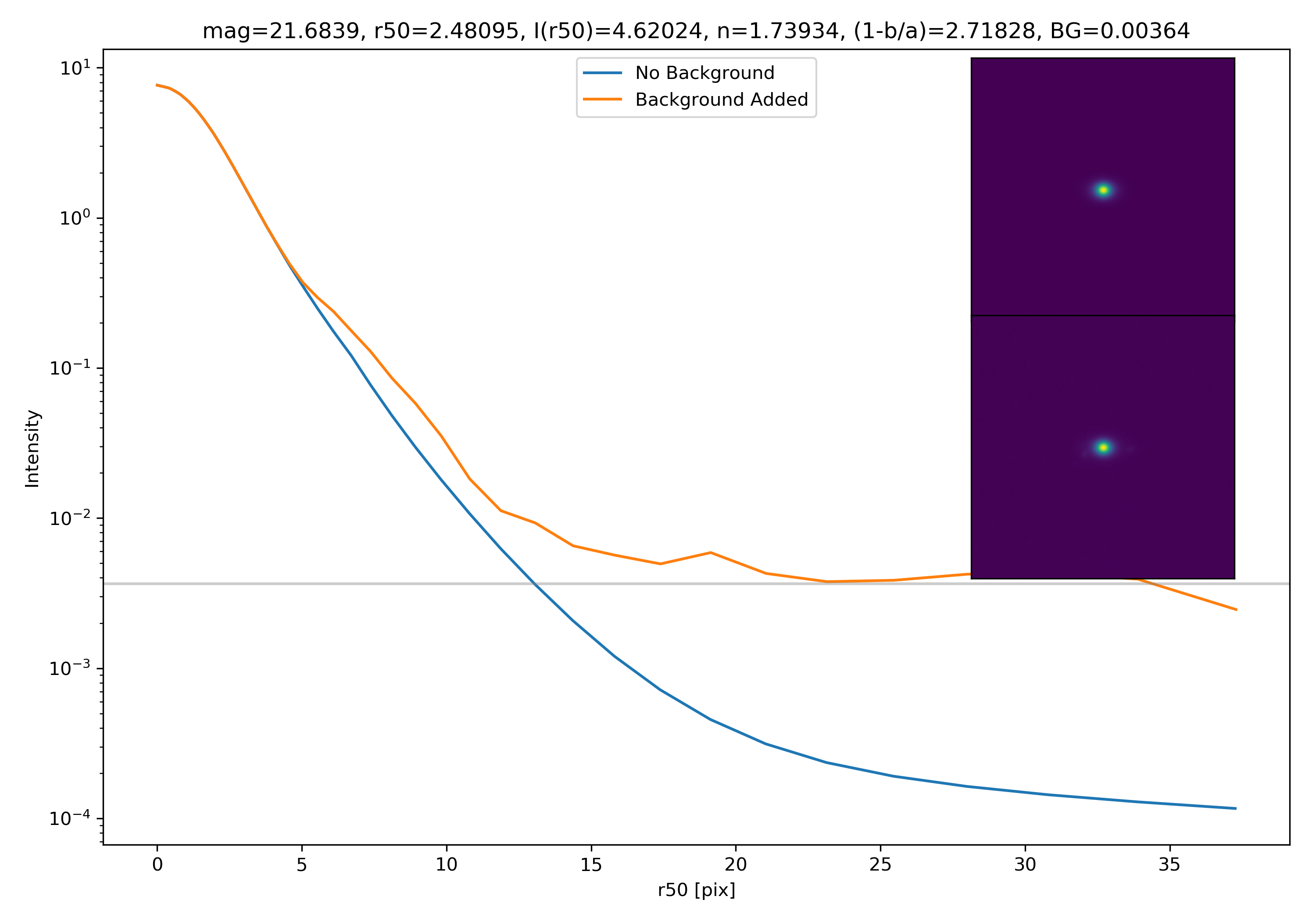
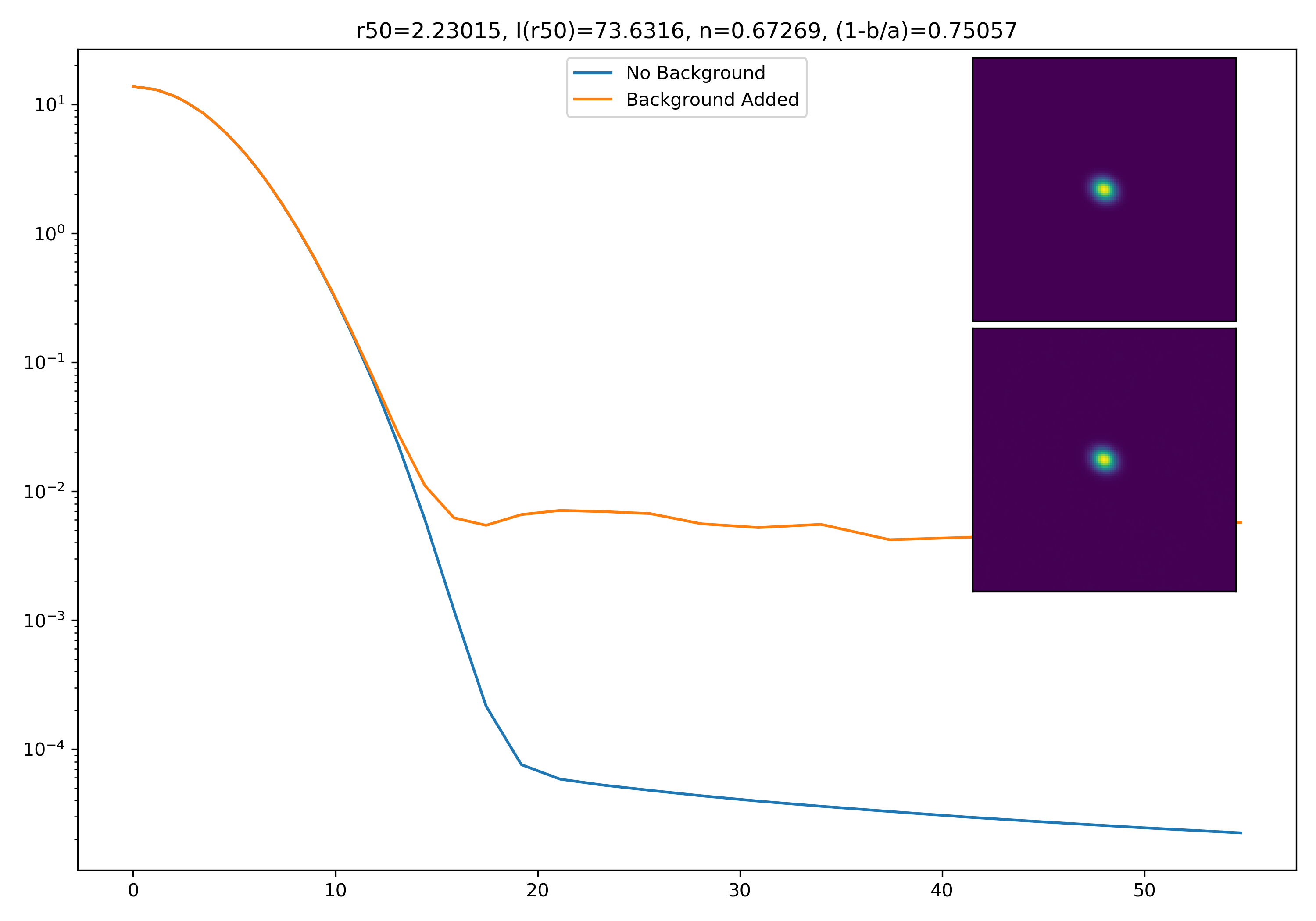
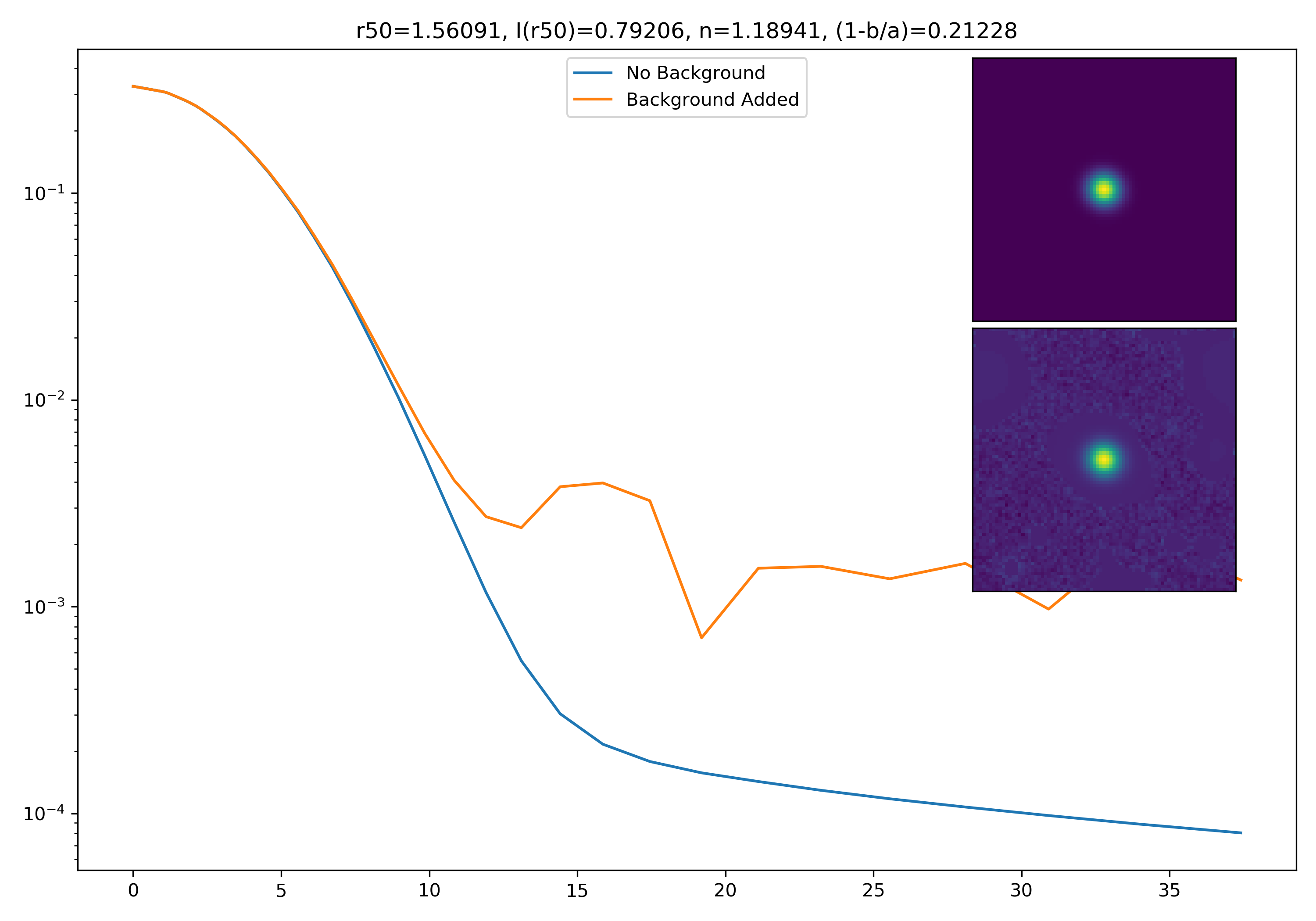
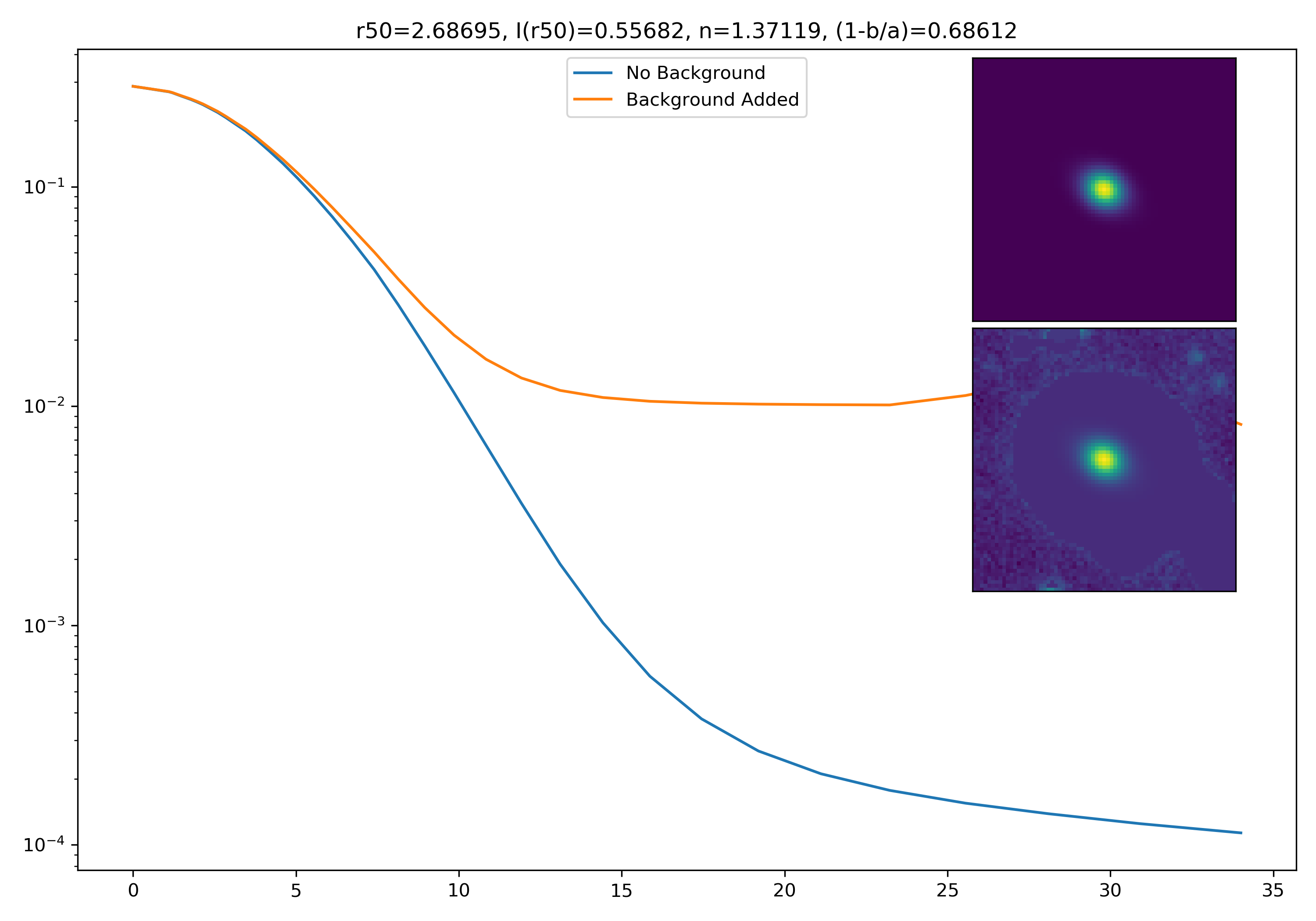
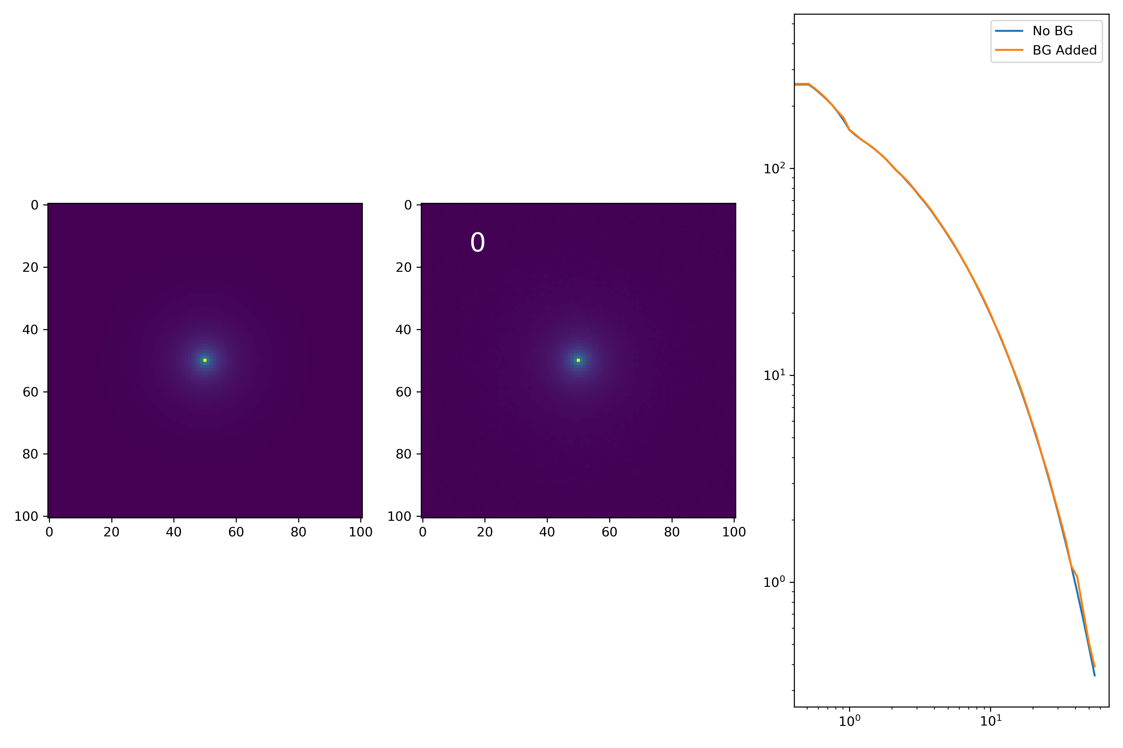
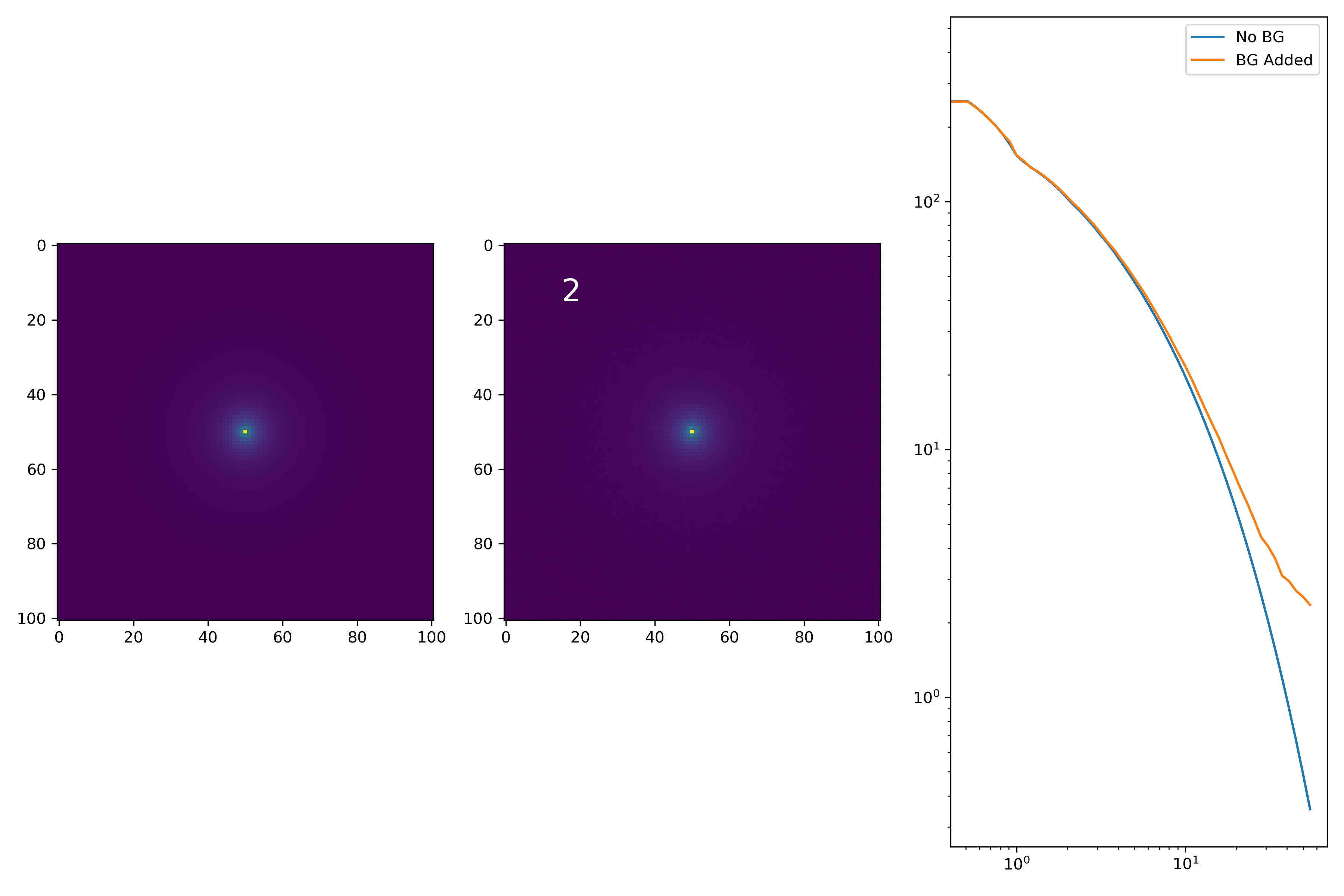
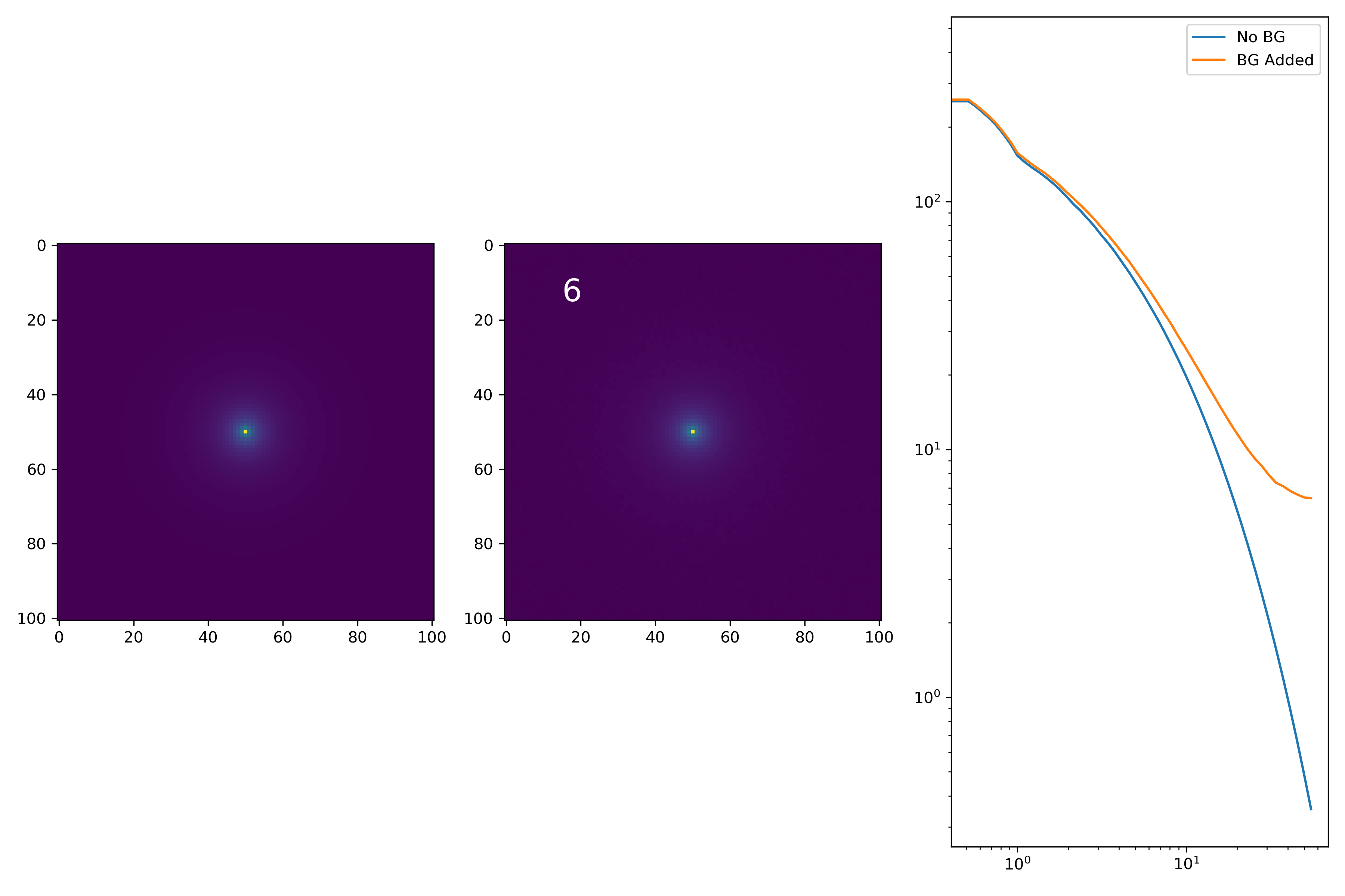
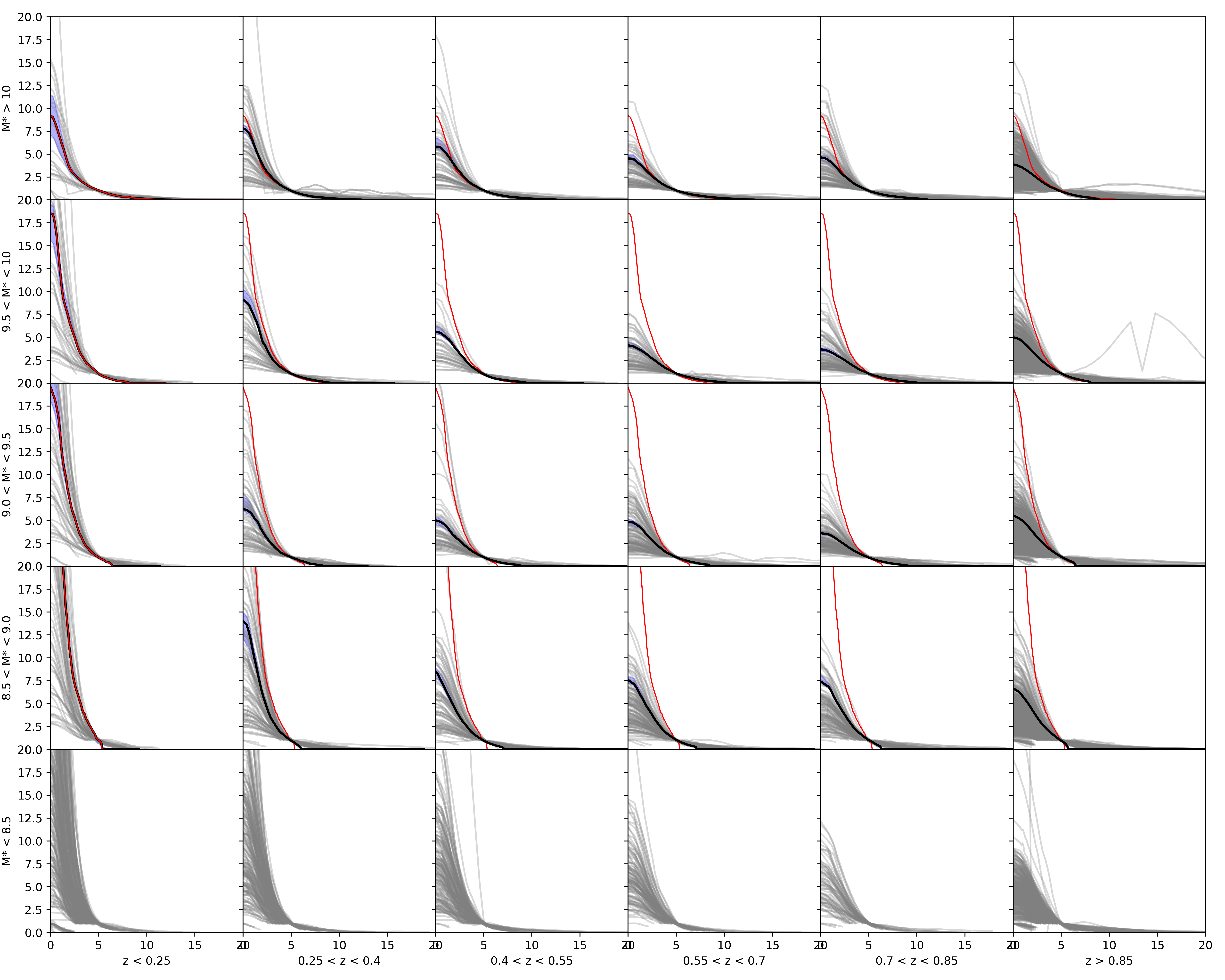
As a final major test for the summer, we want to see how the medians of models differ from medians of models added to the background.
To start tackling this, we simulate models against models placed into backgrounds as before. We only test a subsample of our total, with 0.4 < z < 0.6 and 10.7 < M* < 10.9. This is to simulate this procedure on a single bin. Computationally, this work will have to be done on AceNet when moving towards simulating bins for an entire matrix plot.
I generated 200 models and underwent the same procedure as before. When moving to AceNet, we will be able to generate 50-100 cutouts and simulate these models in these cutouts. Below are the plotted medians. I normalize the median without background to the simulated images. In the lower subplot, I plot the background added median profile divided by the model profile.
As opposed to before, my new method to generate a cutout for model extraction simply involves selecting a random cutout from an input I-Band image. I place the model into the cutout, mask it as before, and fit the profile.
Selecting Model Parameters and Generating Models
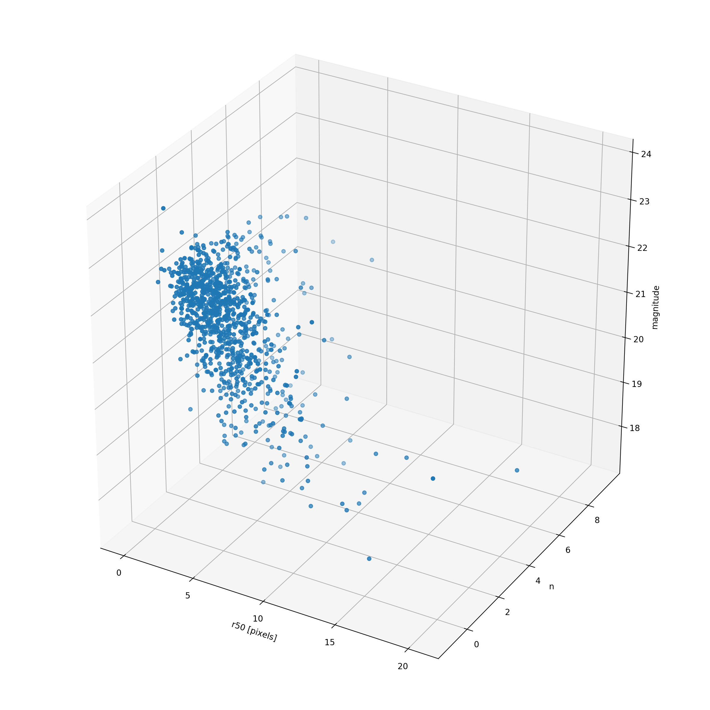
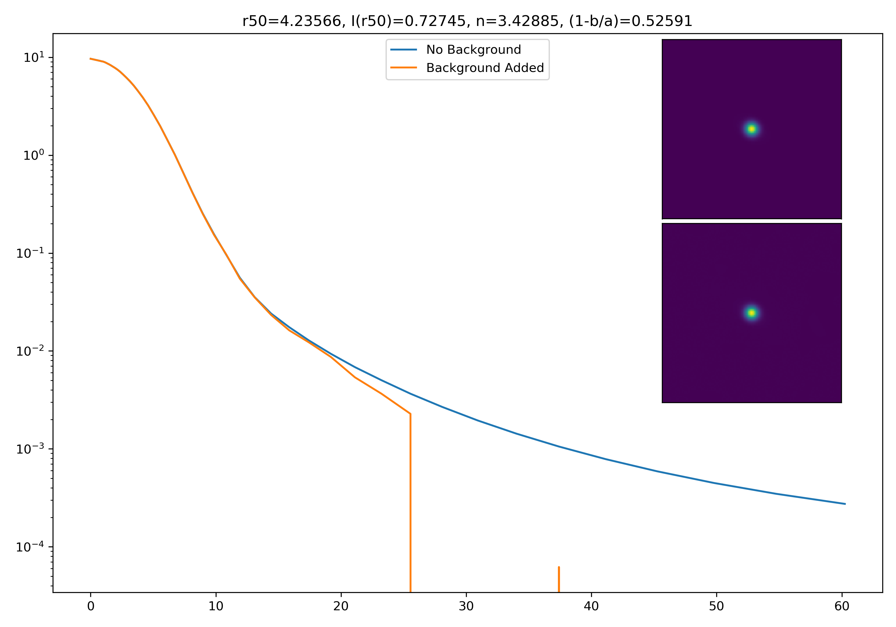
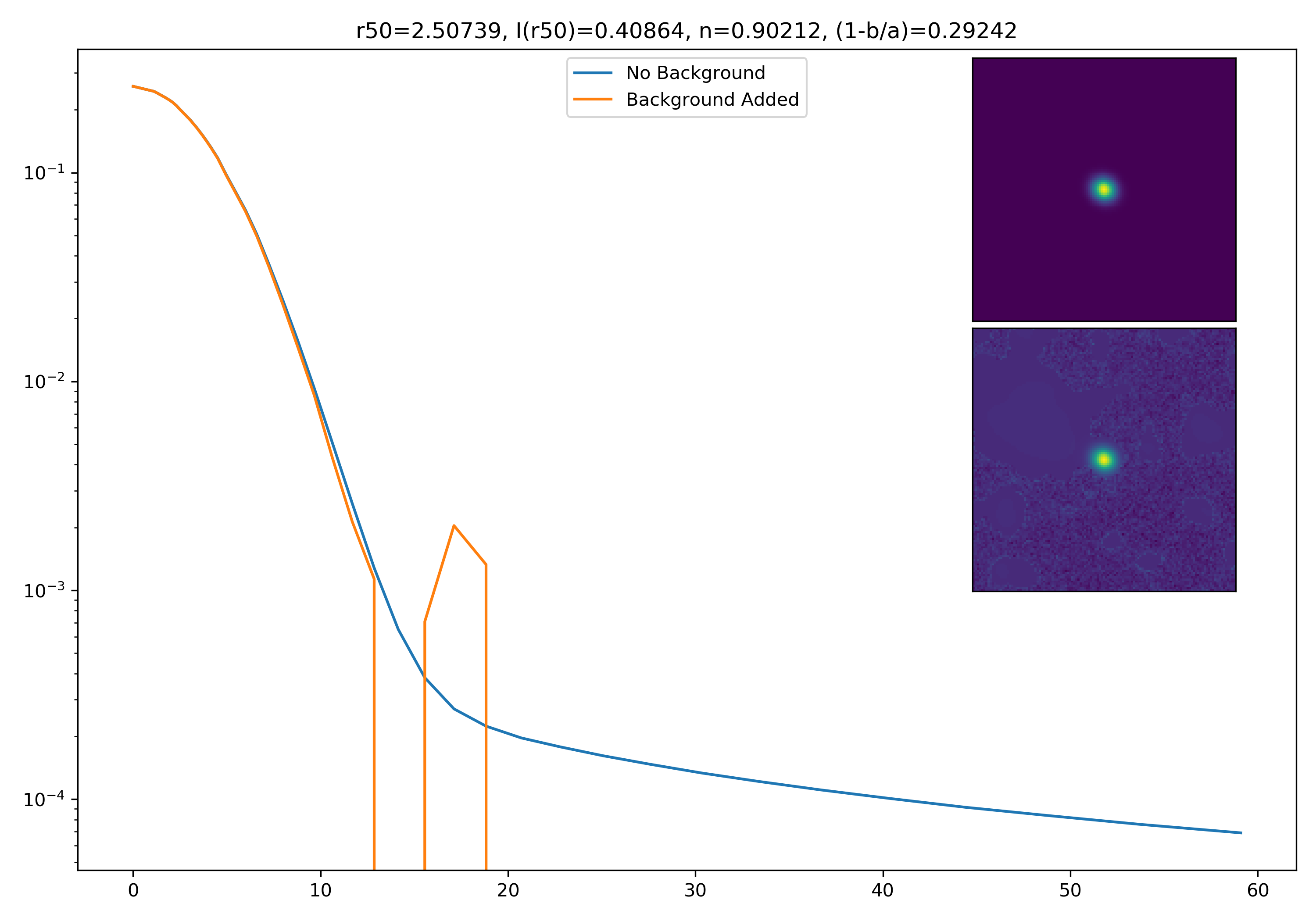
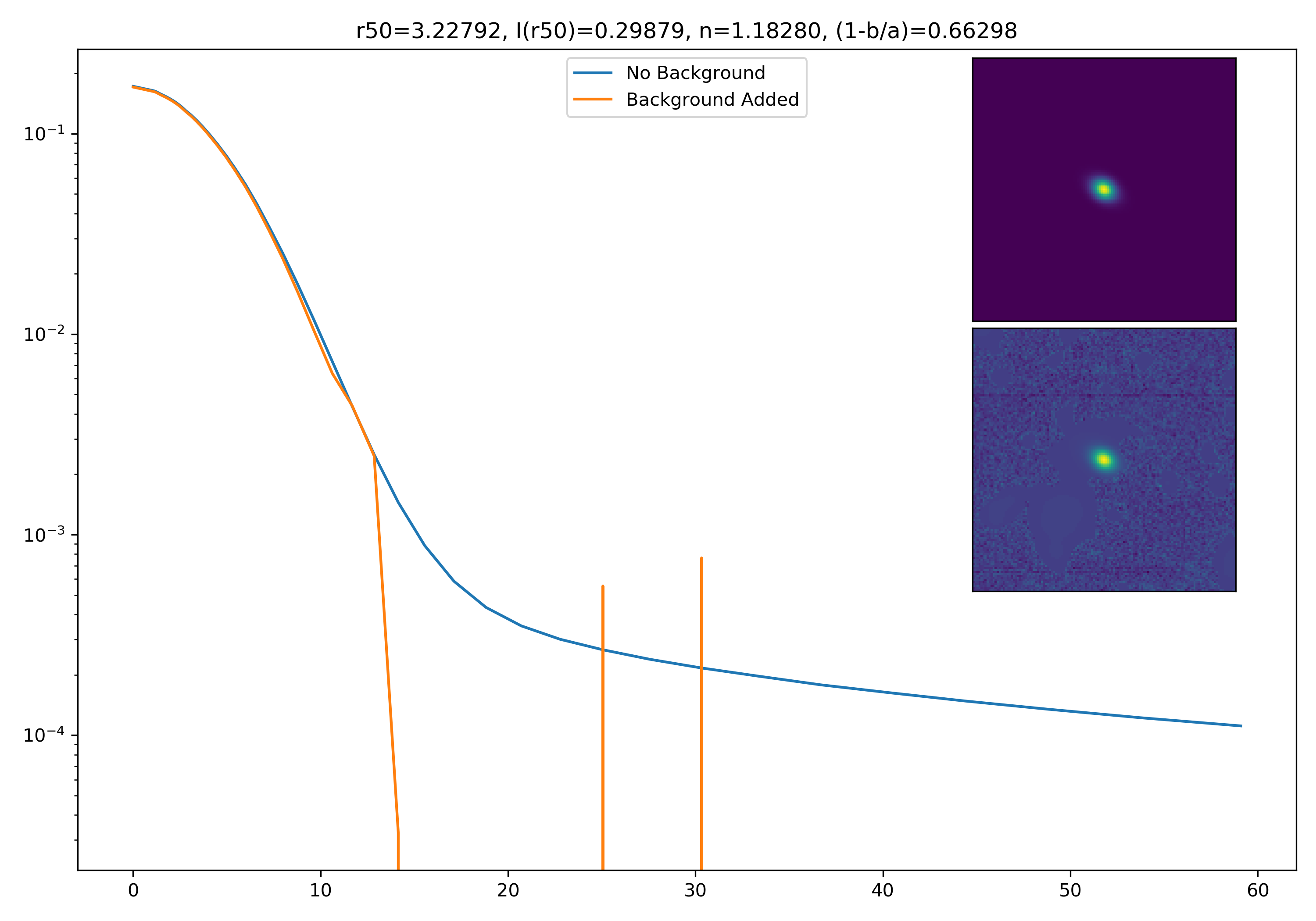
The newest method of selecting parameters involves selecting from n-dimensional space, with the parameters (r50, n, ellipticity, magnitude). Just to check and see where these samples fall, I quickly plotted a 3D scatter plot of effective radius, sersic index, and magnitude. It doesn’t really say too much, but it looks nice (and perhaps would be something to include in the presentation!).
The next step is to generate 2D Sersic models from just the parameters. Using the i-band magnitude, I apply equation (5) from Graham et al. and from that I get the surface brightness at the effective radius. Since there is no scaling that we have to worry about, it’s a simple adjustment to convert SB(R50) to I(R50). We are then all set for model generation!
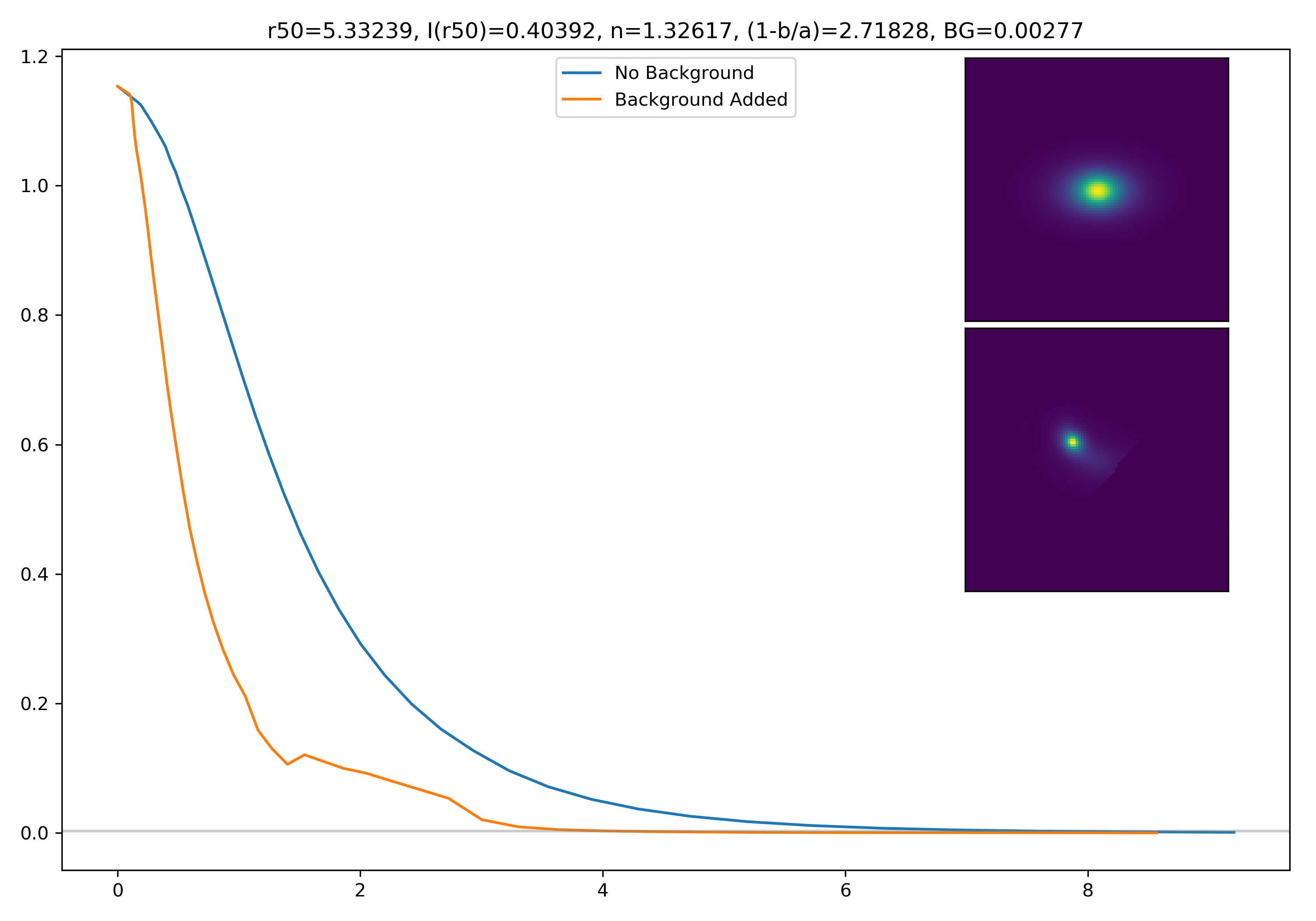
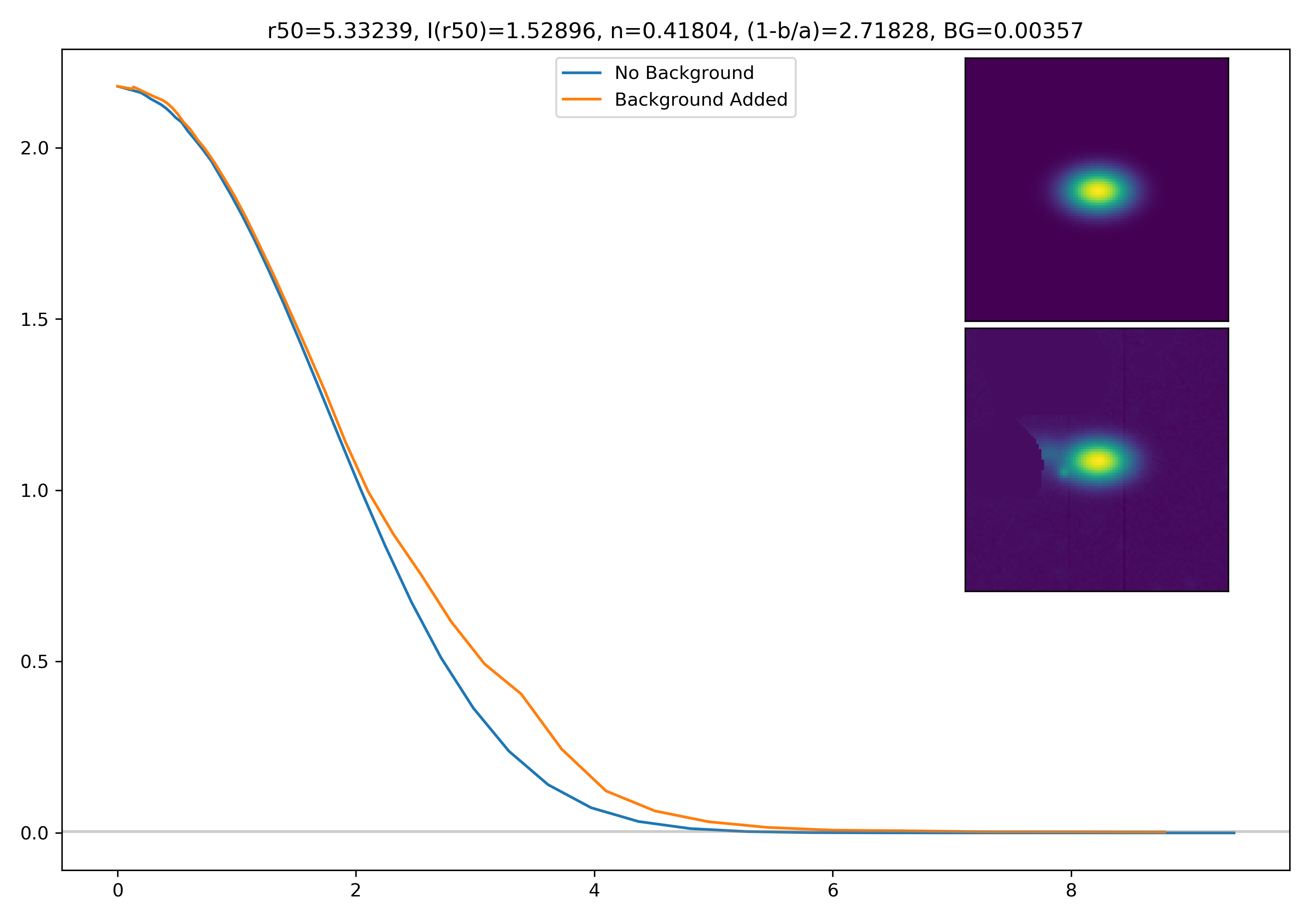
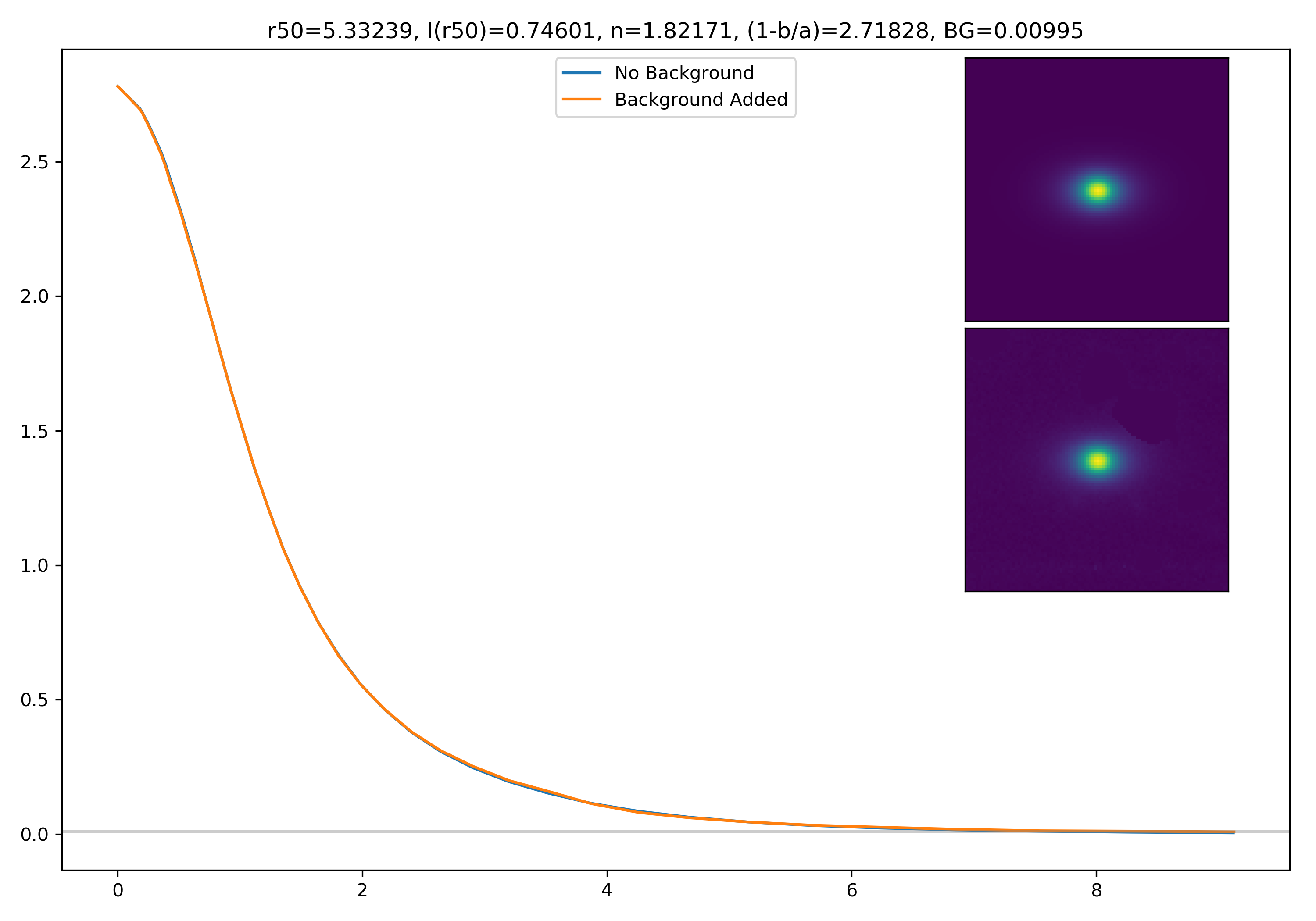
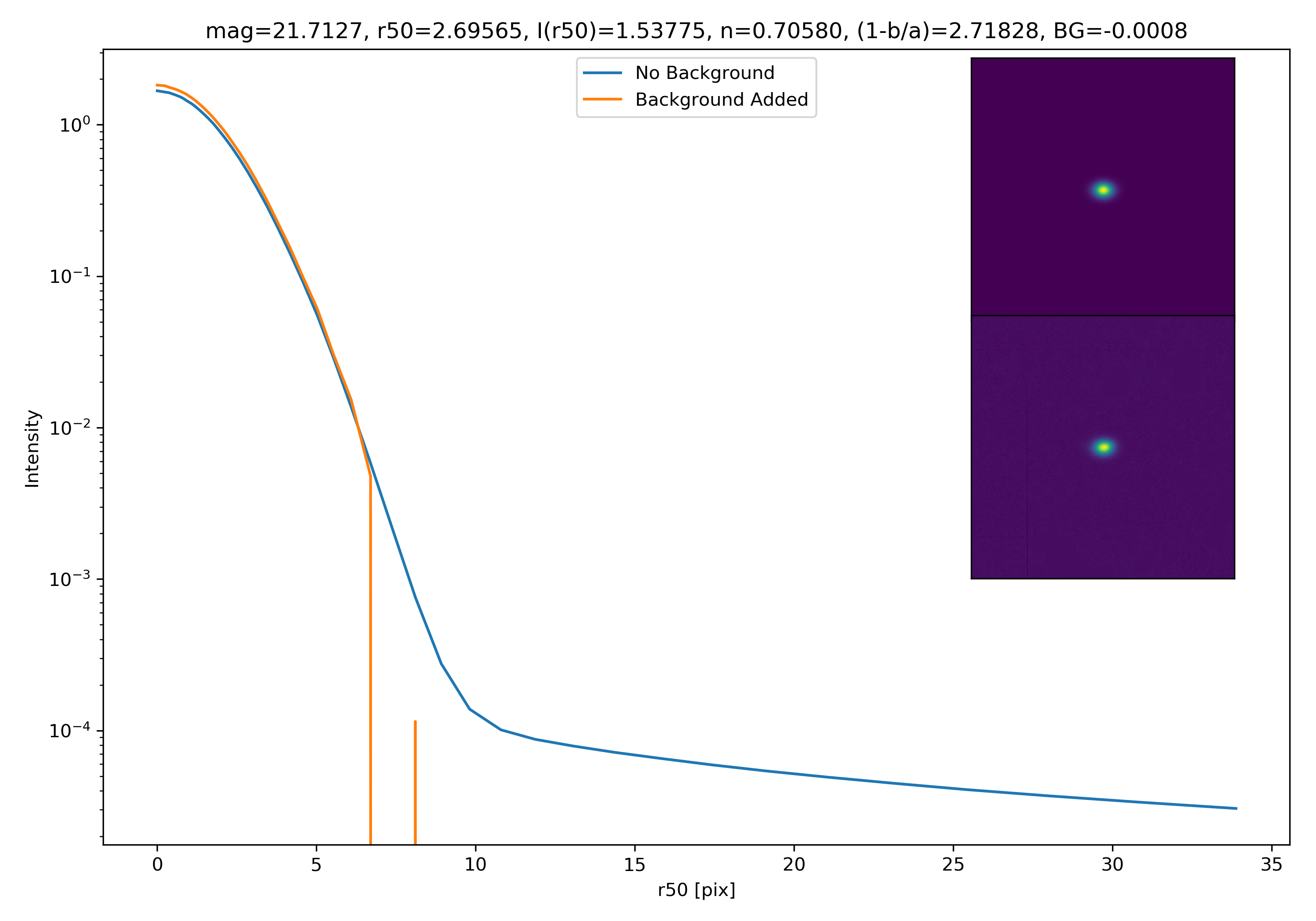
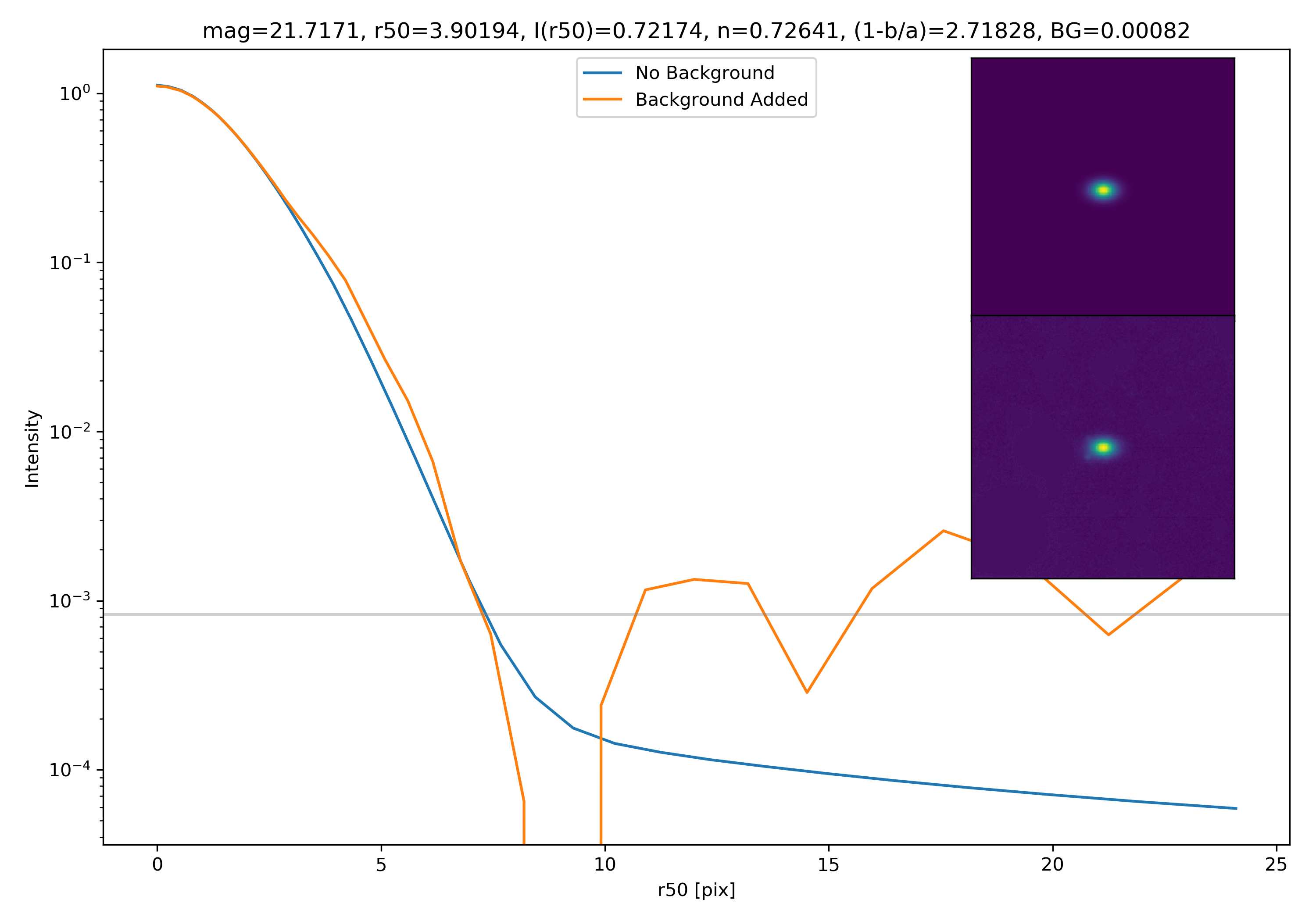
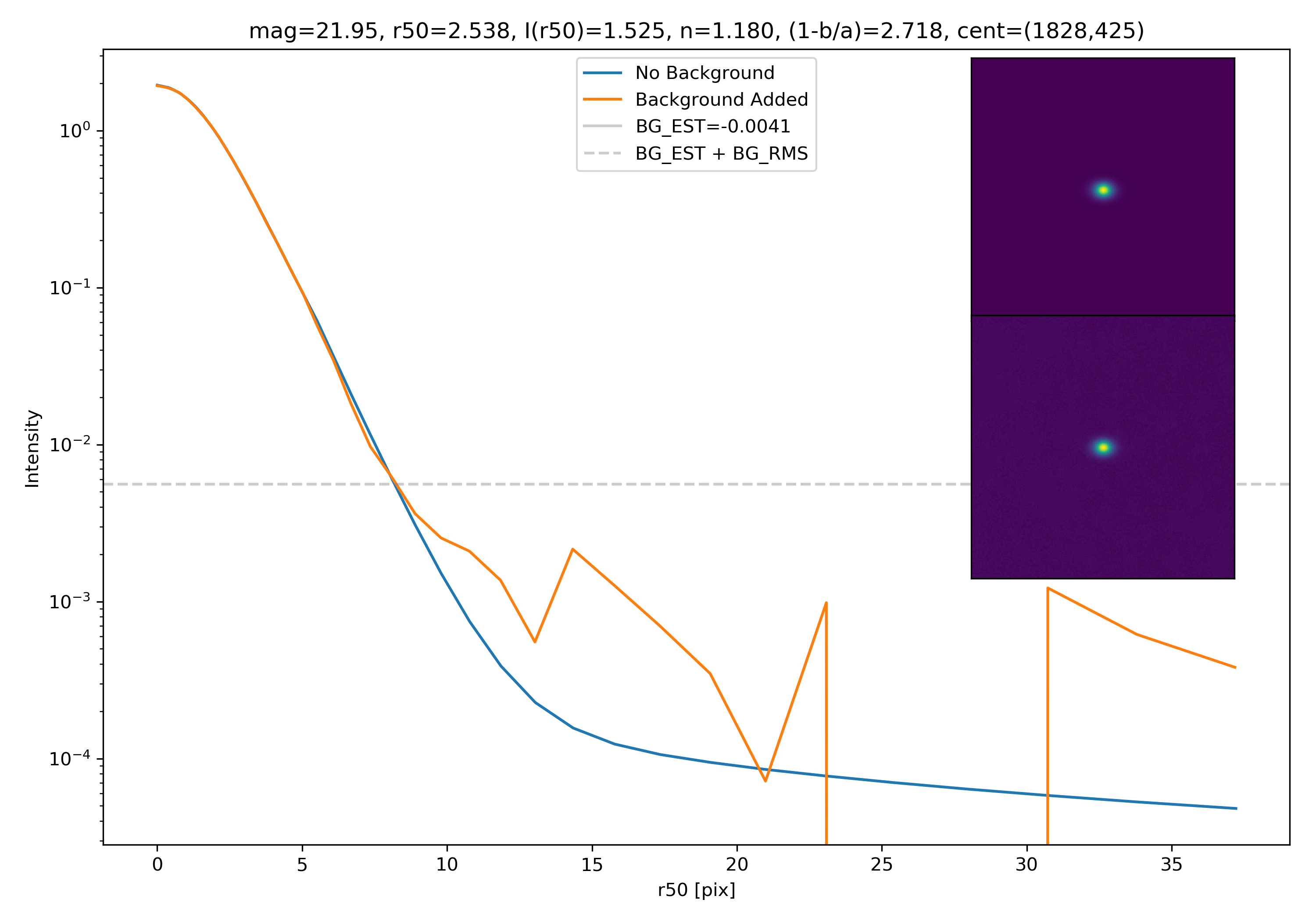
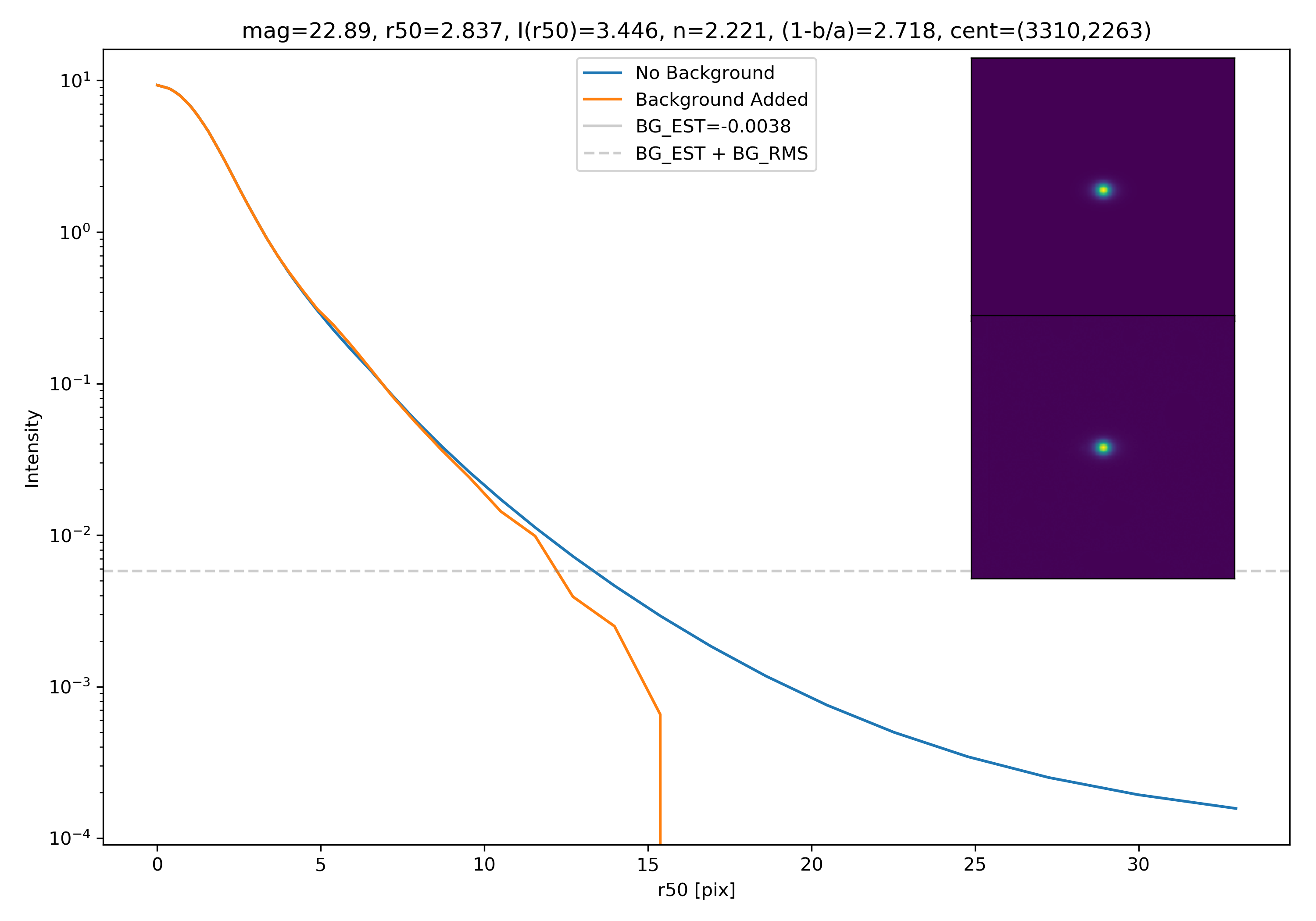
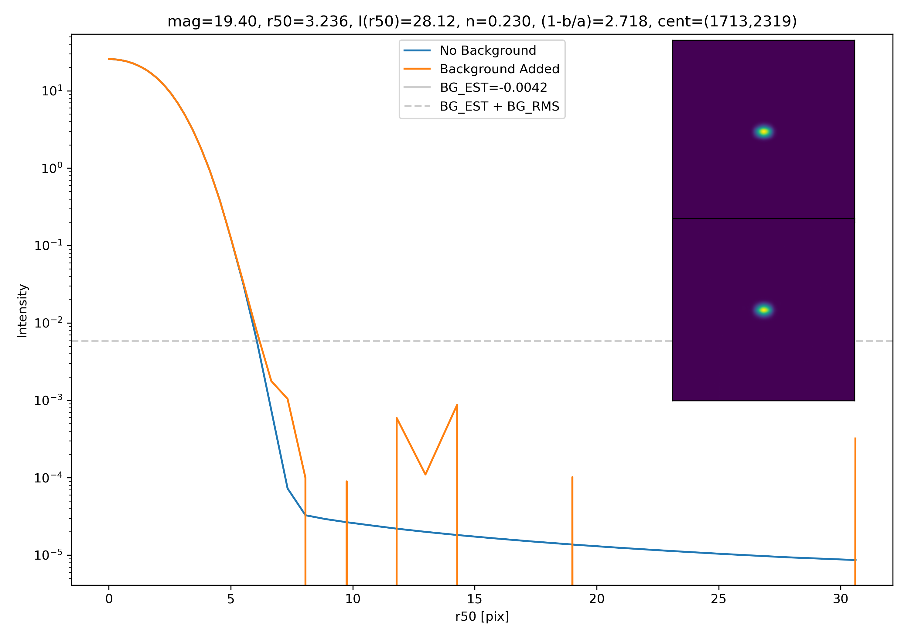
Below are some examples: I grab a random area of the image (200×200 cutout), place the model (already convolved with a Gaussian kernel) into the image, I mask it with the same settings as for profile extraction, and then I extract the profiles of the lone model and of the model with added background. The Grey horizontal line is the background value. However, it’s important to note that since these values are sometimes <0, this line will sometimes not show up due to the scaling of the y-axis. The x-axis is currently being scaled in units of R50.
Fixes to Matrix Plots
I also quickly adjusted the code for the matrix plots. I changed it so that individual profiles are plotted bin by bin (as opposed to before the median calculation), so the medians are definitely being plotted in the right place.
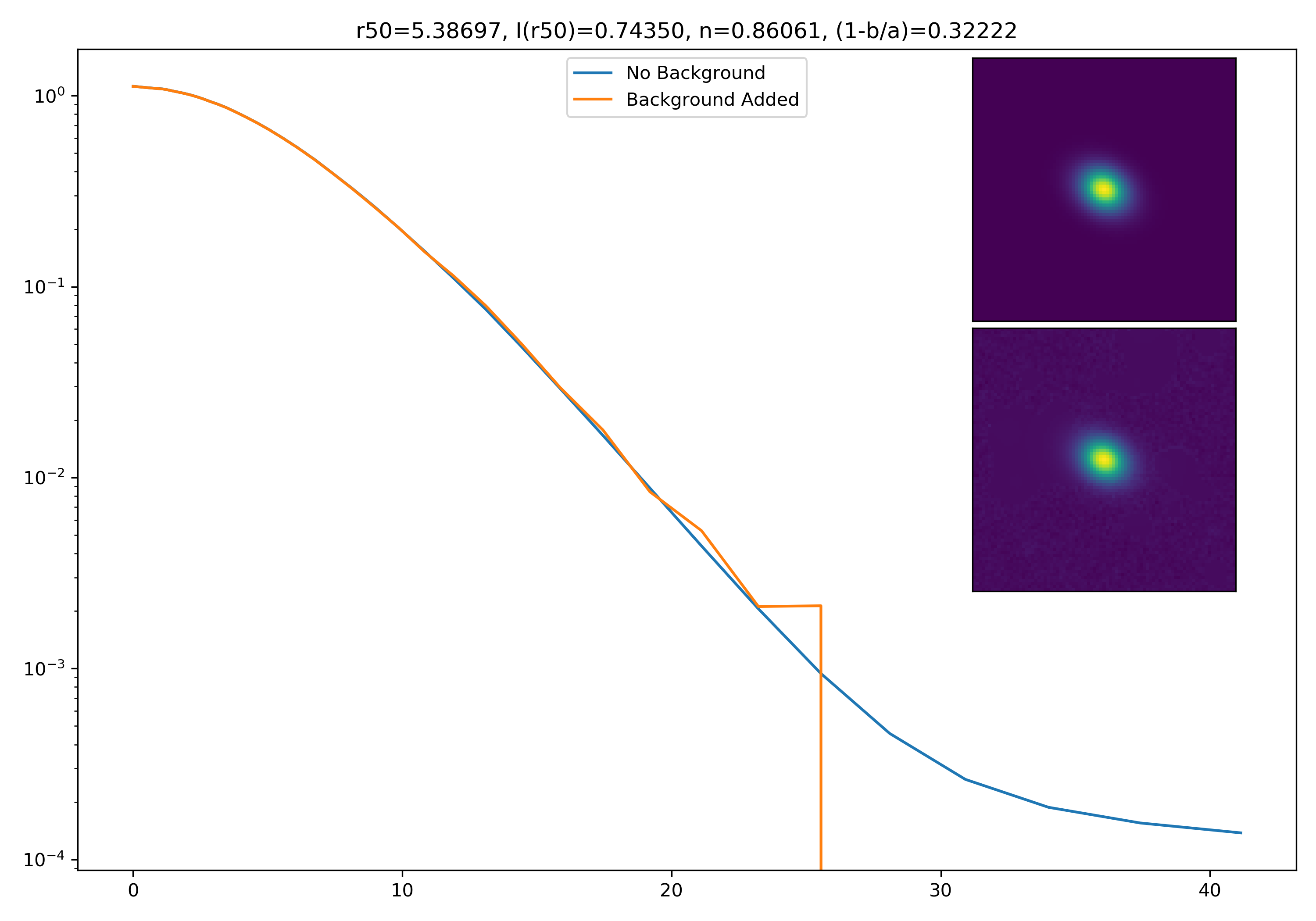
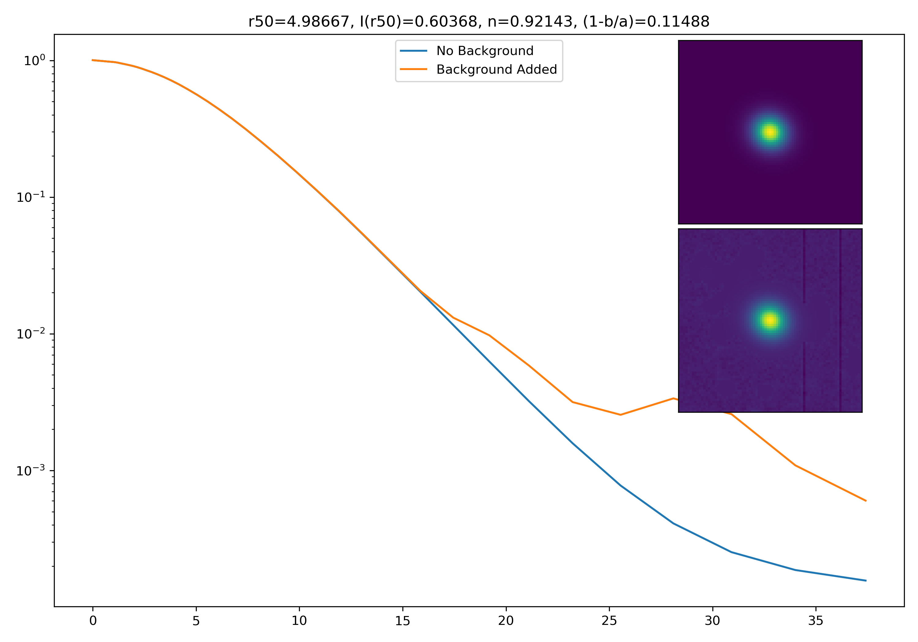
Updated Models
Here are some updated models with the following adjustments: – r50 actually varies properly – no normalization
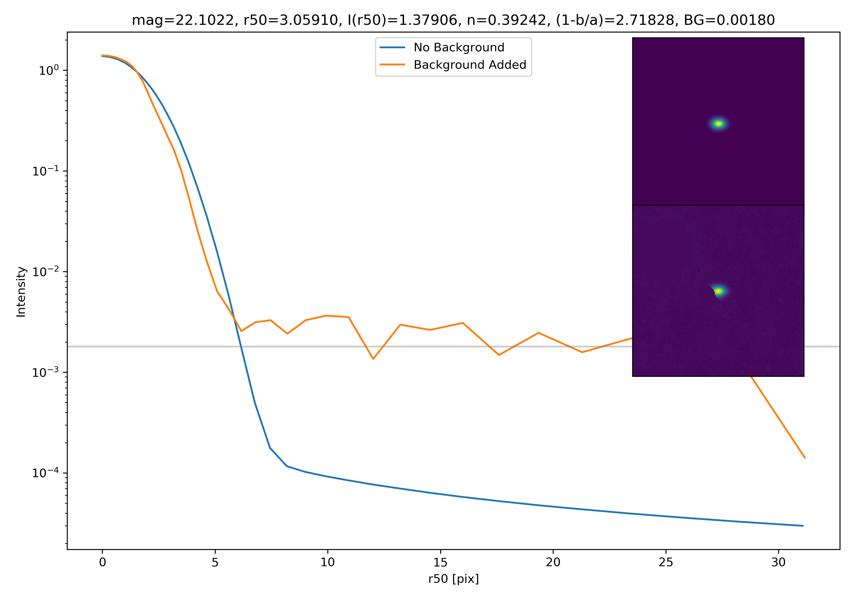
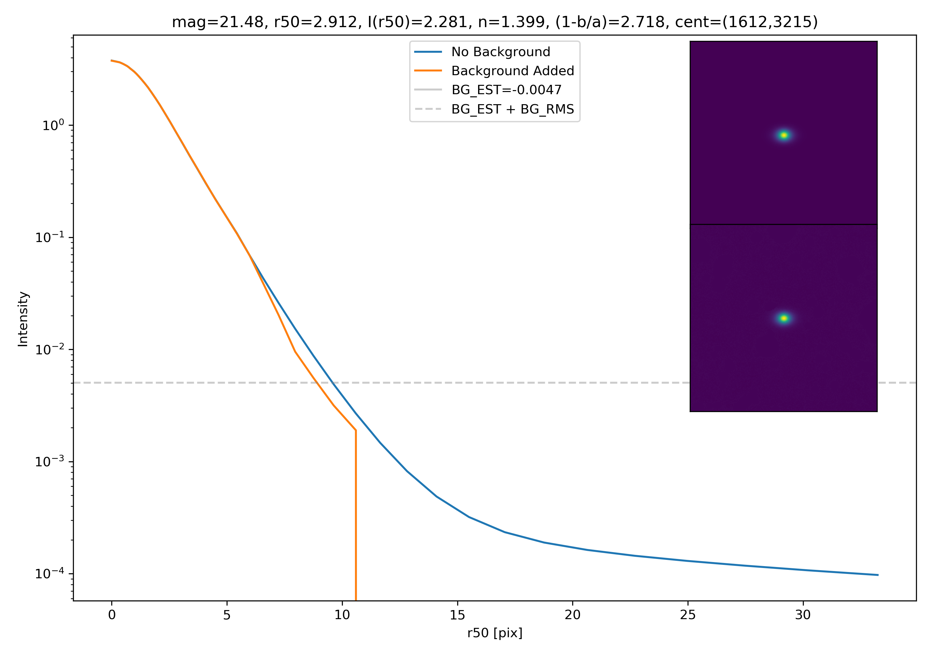
Models with Root-Mean-Squared Background Noted
To get a root mean squared value, I use the super pixel from which the background is taken. I square all values in the super pixel, take the mean, and then the square root of the mean. That value added to the background estimate is plotted as a dashed line. Below are some examples.
If I had to say, I think that considering this value as our cutoff point is not a bad idea! A lot of divergence from the model tends to occur close to when the model added to the background passes this value. Especially if the background estimate is negative!
Here are the updated heatmaps for the u and u* band. The issue was indeed with the tick marks, and the bins have ranges of 0.2. The problem with the heatmaps was I likely wasn’t grabbing enough of the good/bad ids. It’s possible too that I was grabbing say, the file containing unsuccessful IDs for a tract and not the file containing successful ones. To prevent this issue from happening in the future, I am gonna change the output file containing successful/unsuccessful ids to be one file in a table format, with one column being the ID, and the other being with “S”/”U” to denote how the extraction went.
These are the updated ratios and totals for the u band.
And these are the updated ratios and totals for the u* band.
Fixed Convolution Bug
The old way that I was trying to convolve was to generate a 2D Gaussian (with the same image shape as the 2D Sersic profile). I would then use the standard convolve method previously used. This was returning a strange vertical spike of brightness through the centre of the convolved sersic, and I admittedly had no idea how to fix it.
To circumvent this problem, I attempted to use astropy’s convolution package. Instead of a 2D gaussian image, I generated a 2D Gaussian Kernel with an adjustable standard deviation. When I convolve the 2D Sersic image with this Gaussian Kernel, the convolution works properly.
Before being placed in actual environments, you can see a much more faithful looking model.
Modelling, Continued
Lots of things to learn for the latest meeting!
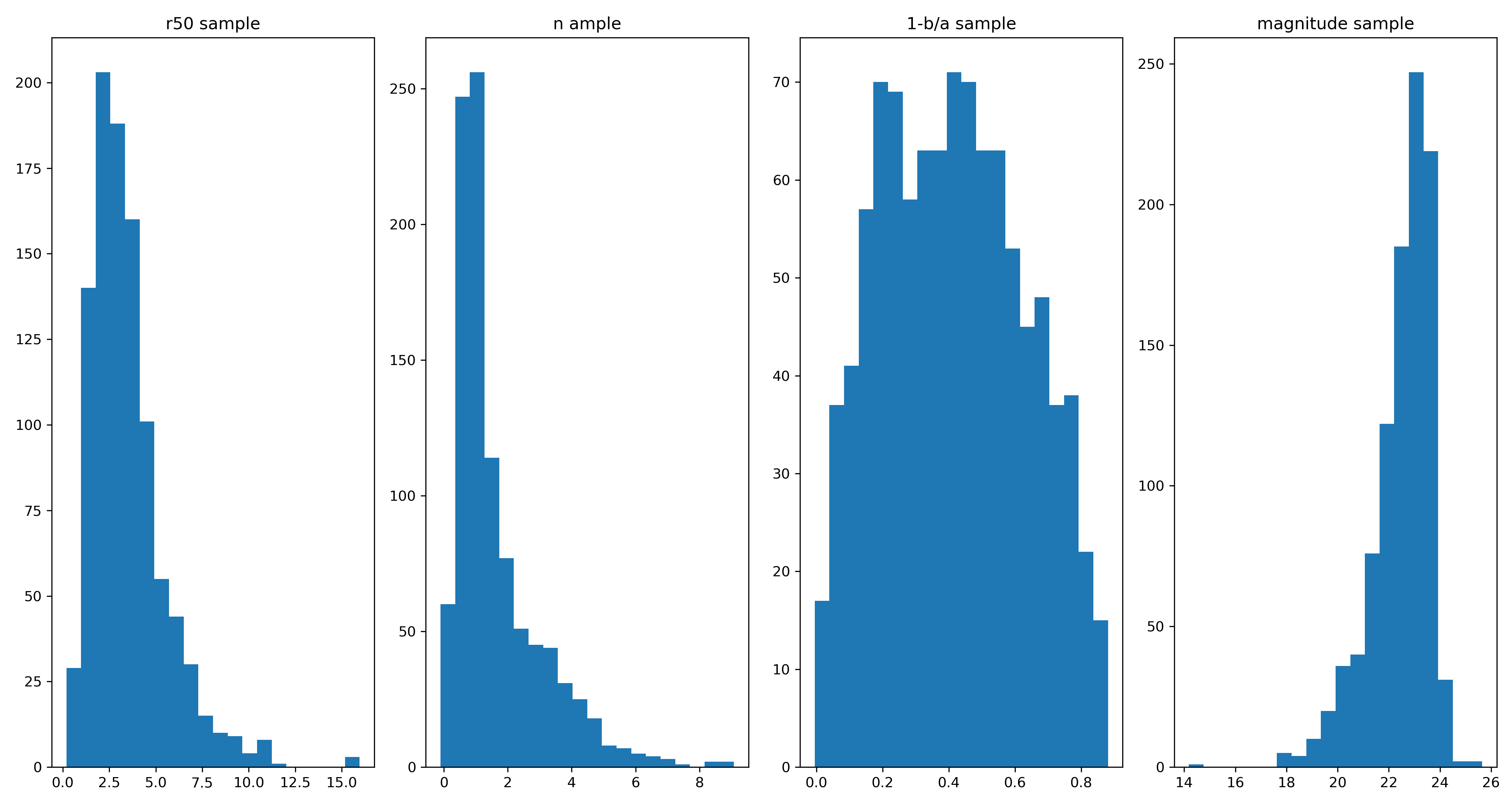
Ivana requested that instead of just choosing arbitrary parameters, I use the galaxies we already have and some of their morphological parameters to justify our model settings. I had to learn what the two functions Ivana linked did.
To my knowledge, this is what they do. The first method is to generate a probability density function (PDF), which would be loosely akin to fitting a Gaussian to a histogram. Once we have this PDF for each parameter, we can use this to sample model parameters. The figure below shows the histograms for 1000 samples for model parameters.
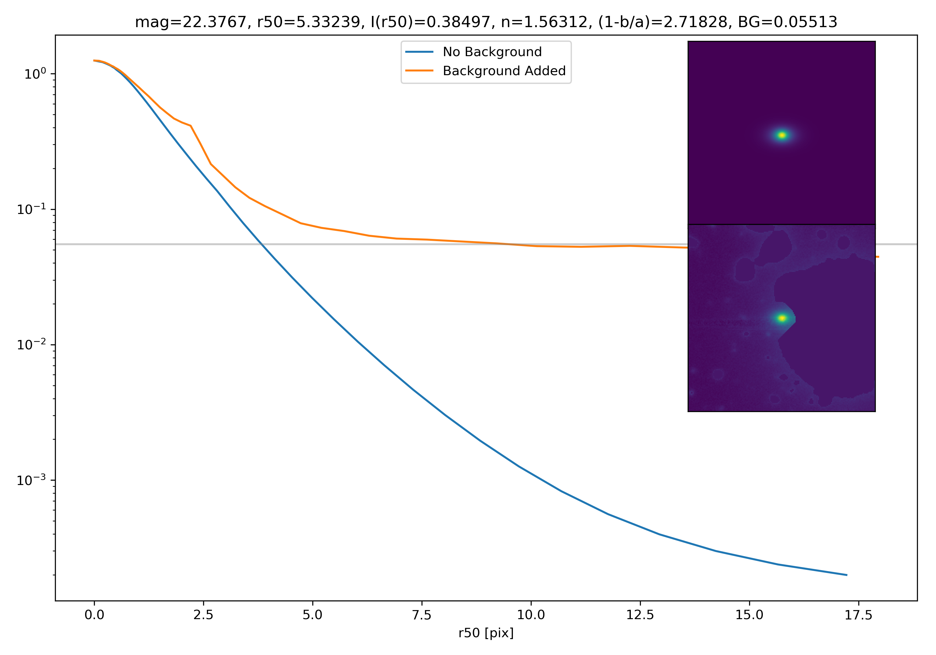
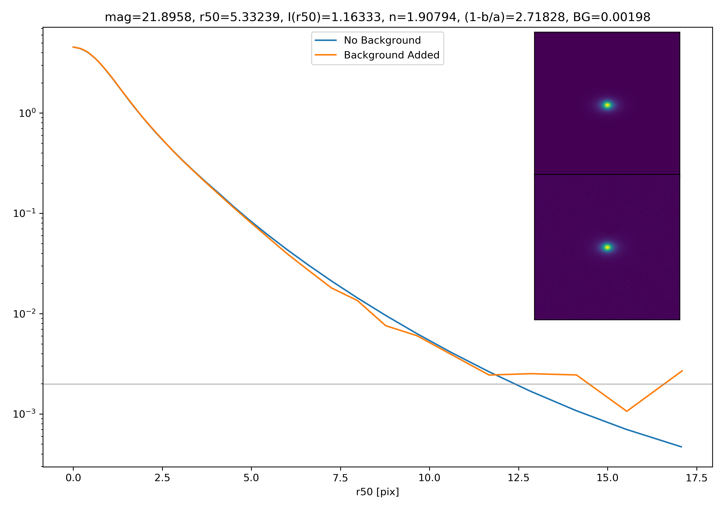
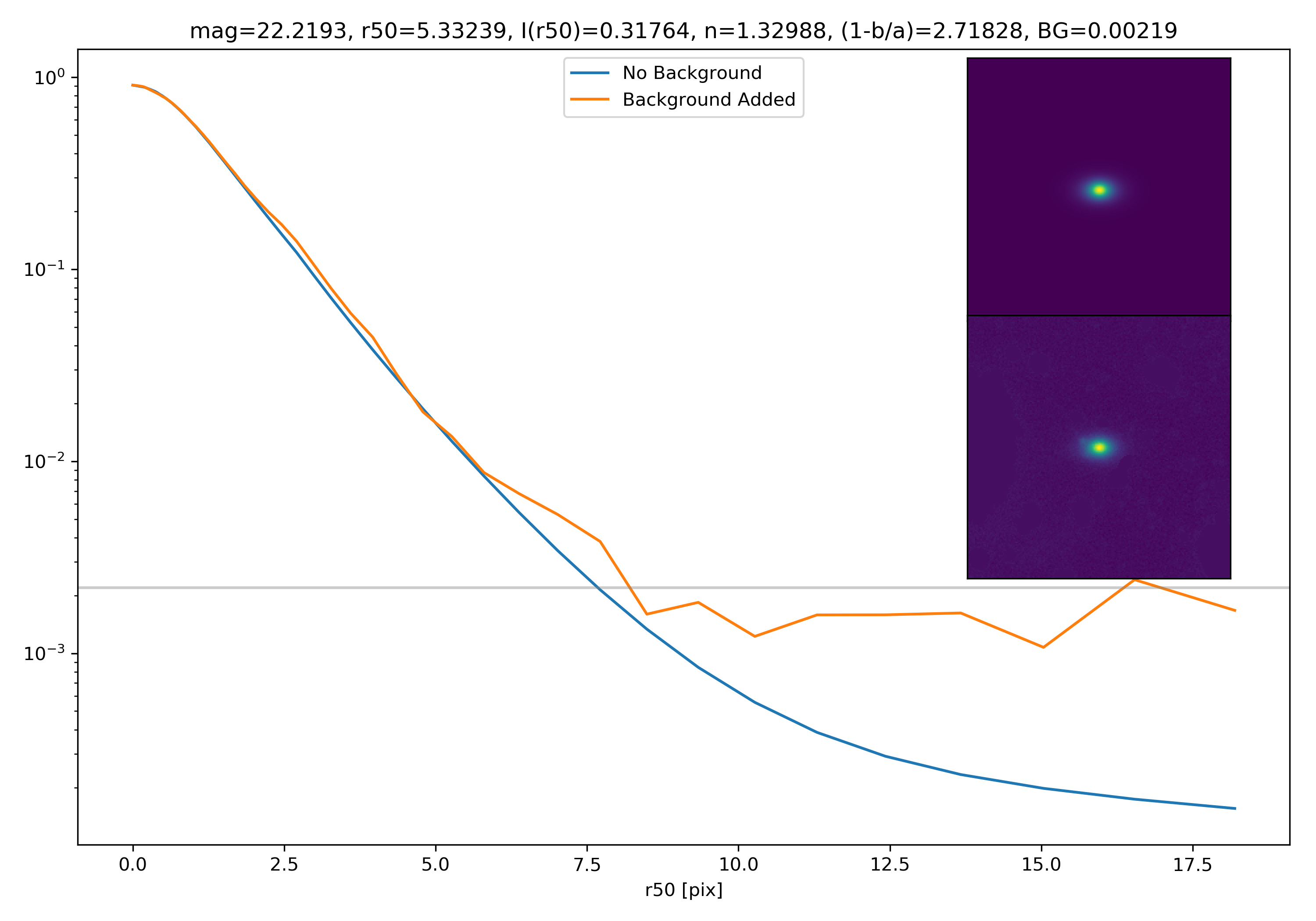
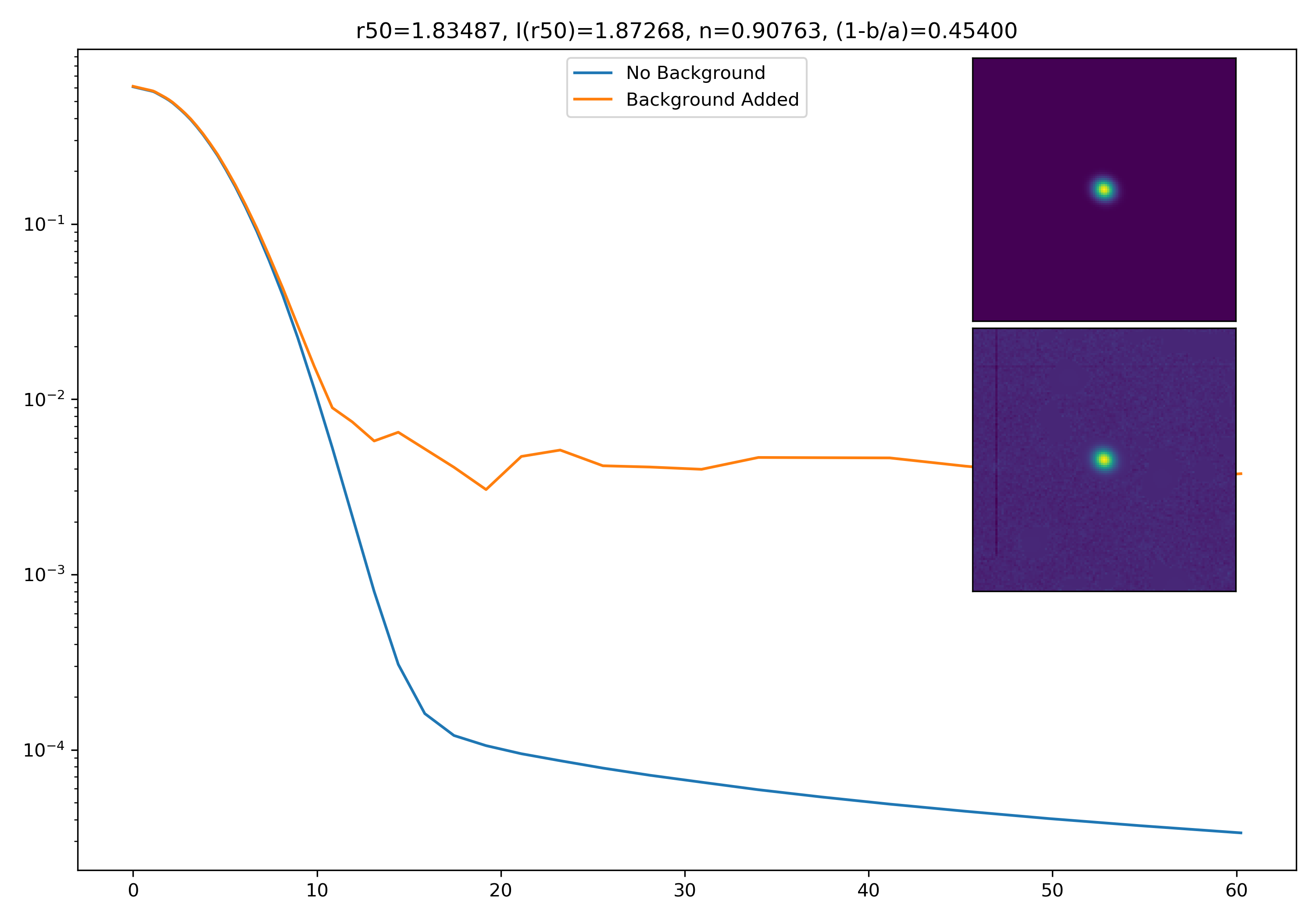
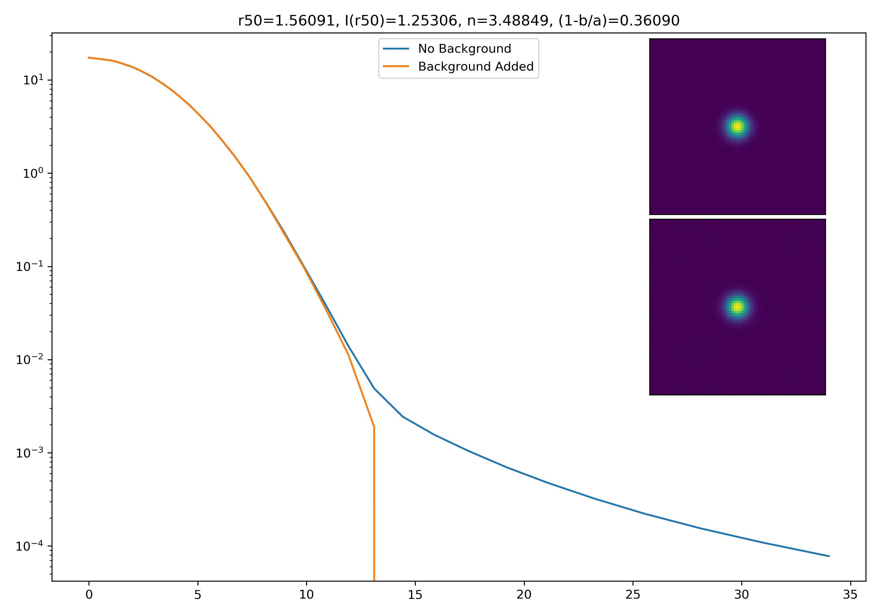
From these samples I can choose parameters at random using numpy.random.choice(). I can then easily generate model profiles. For backgrounds, I do aggressive background masking to simulate a sparse region for 200 cutouts. I also get the intensity at HLR for 200 different profiles. This is so I can scale the model properly. Using all these parameter choices, we can generate profiles however we want. Below are some examples! The parameters are also included on the figures.
Interesting results! As you can see, there are two noticeable effects. The first is that the profile is “peeled up” if the background is somewhat bright. However, since I’ve logged the yscale, if it enters a region of I(r) <= 0, if drops down heavily. One it hits those the profile starts to get a little crazy looking.
Here are the heatmaps for all bands! As you can see, some bands seem to fare better than others. One thing to note is that I don’t think the ratios in the high-redshift region of the r-band are accurate. I noticed in the totals that there are few objects in that region, so it’s likely the pipeline just got lucky with a few.
g-band
r-band
i-band
z-band
y-band
u-band
u*-band
Modelling
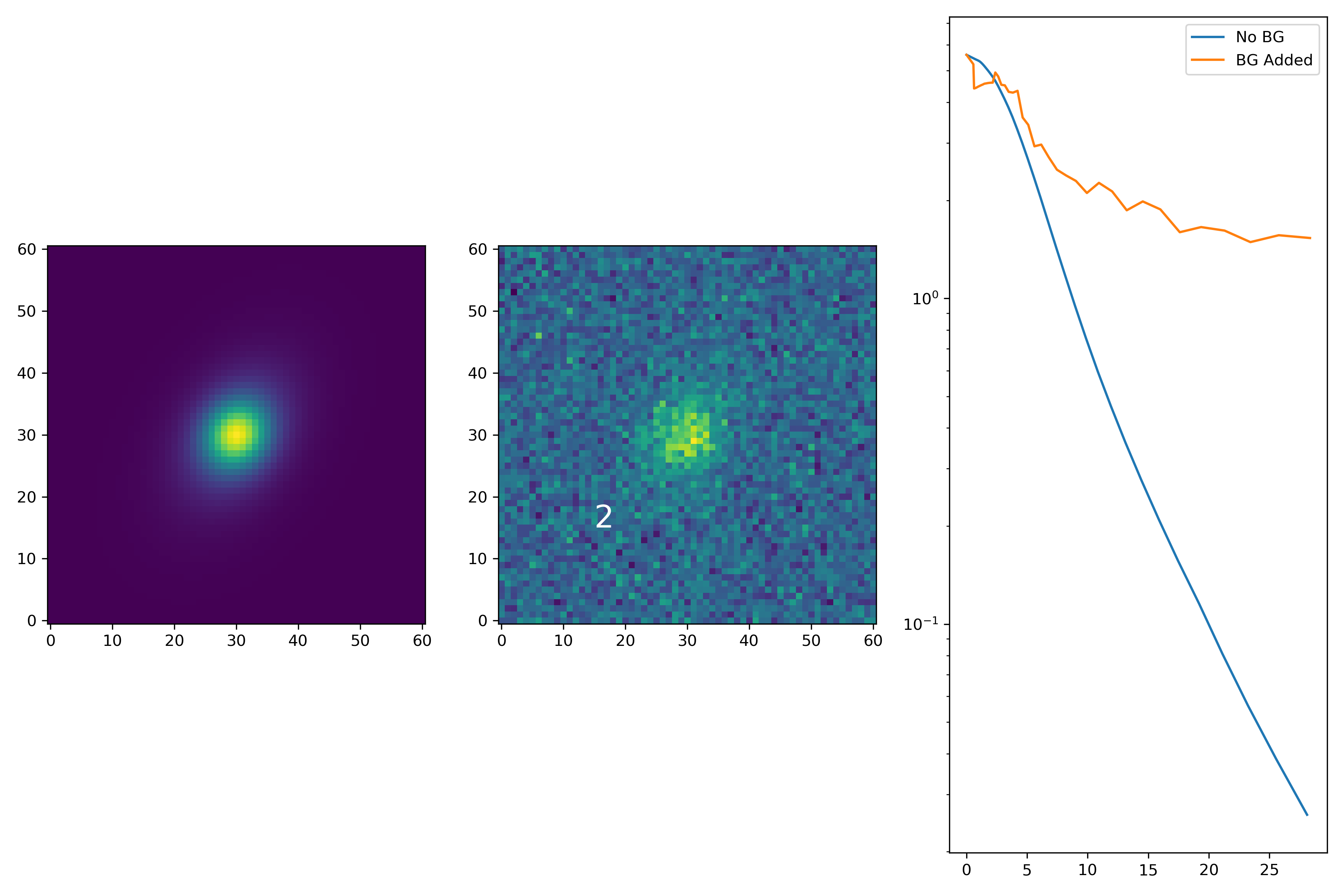
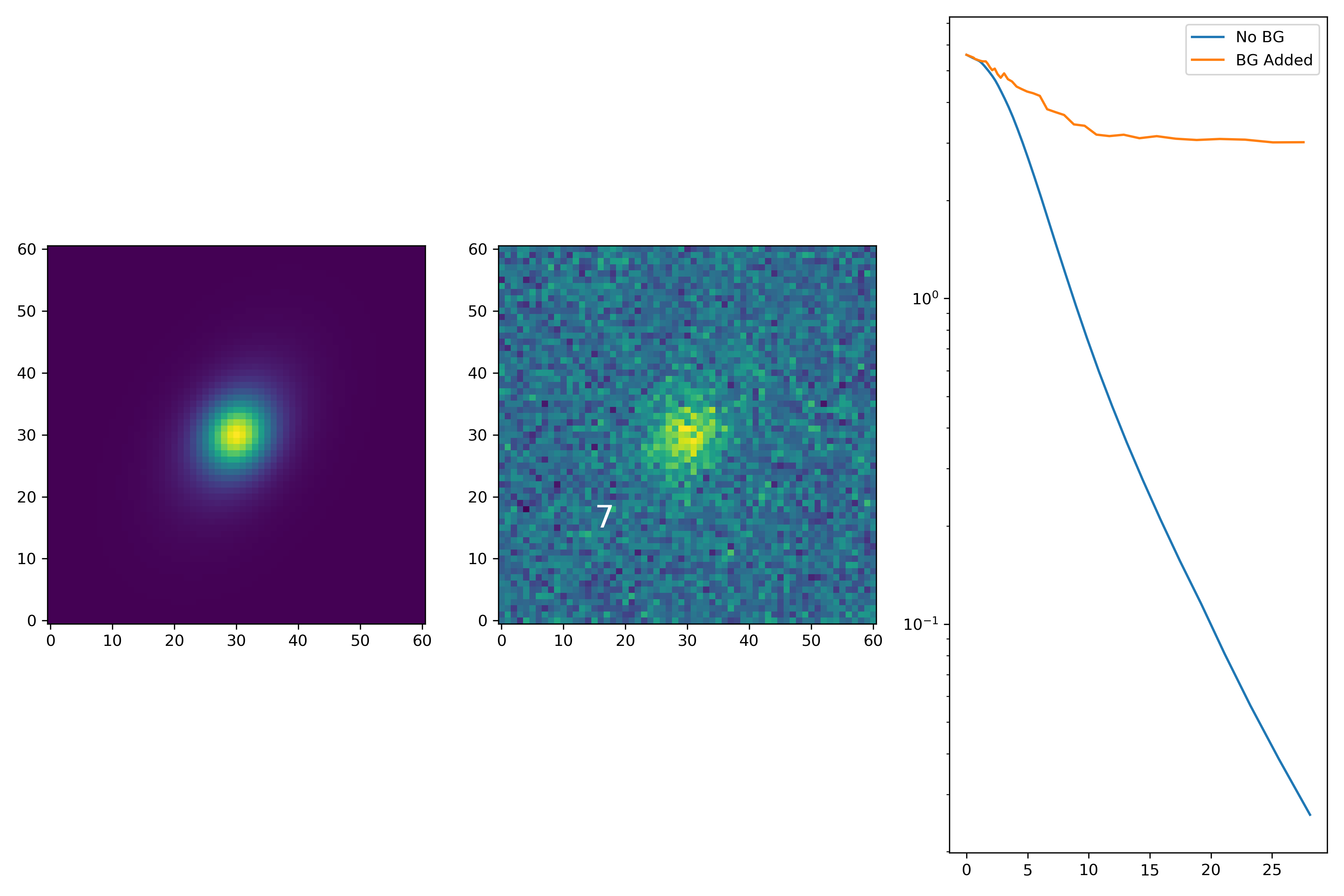
To test modelling (properly), I generate 2D Sersic profiles with n=2. I noticed when convolving with a 2D gaussian that the resultant models had a strange “spike” in the profile. Since I wanted to test the effects of the background on the resultant profile, I decided against convolution (for now until I can work out this bug) and decided to increase the effective radii of the profile.
I test increasing levels of background, and I also simulate noise using the photutils method make_noise_image. I then fit the profile without added background, and fit the profile with background added. These following plots show cutouts for these two profiles, along with the normalized profiles.
The cutouts don’t really show much (due to the scaling of the cutout), however, you can see the profile being “dragged up” in the rightmost figure.
NOTE: These figures are just to get a general sense of the role the background plays on a typical profile. It is not actually measuring anything related to the galaxies whose profiles we have extracted.
Profile Extraction Parameters
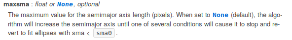
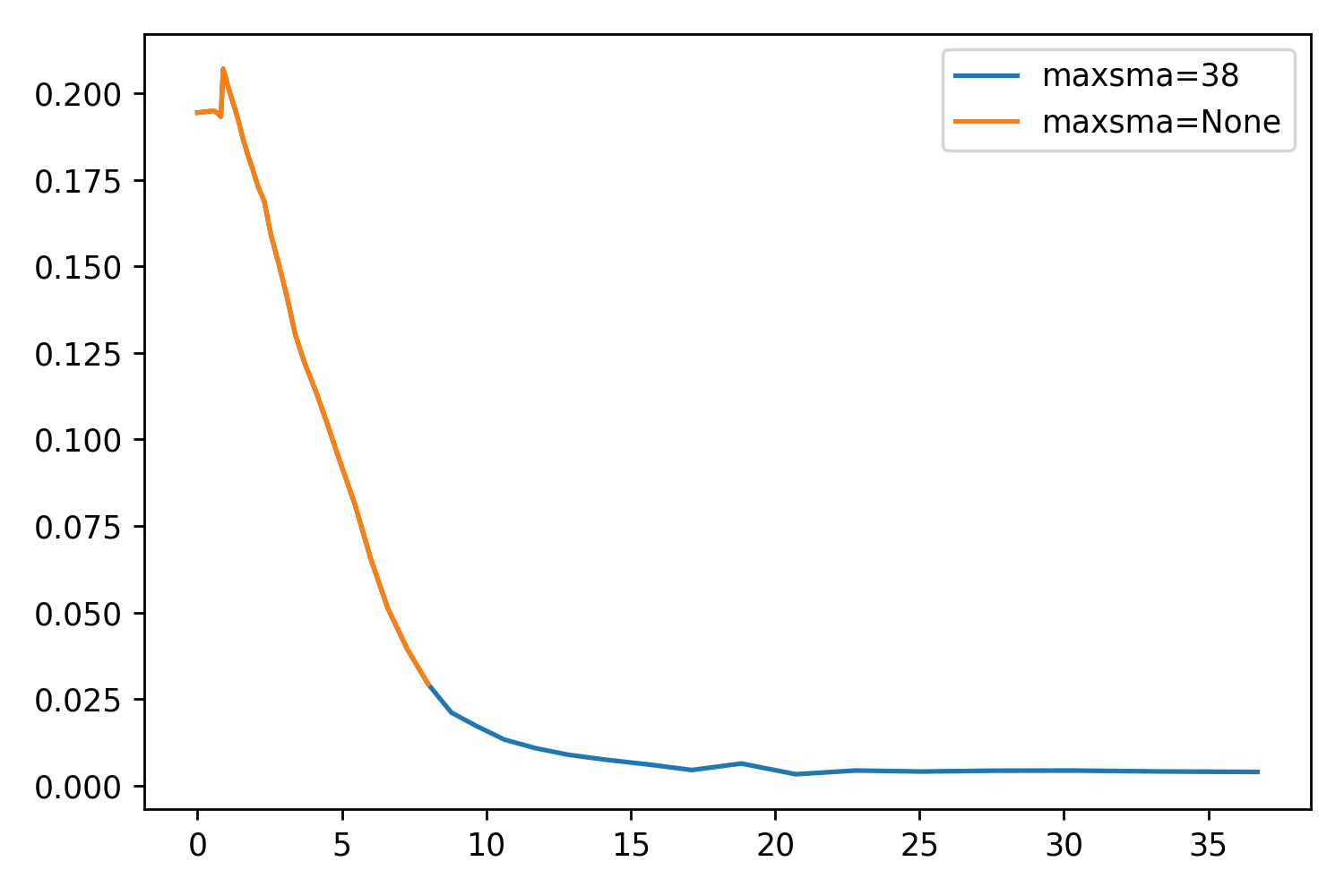
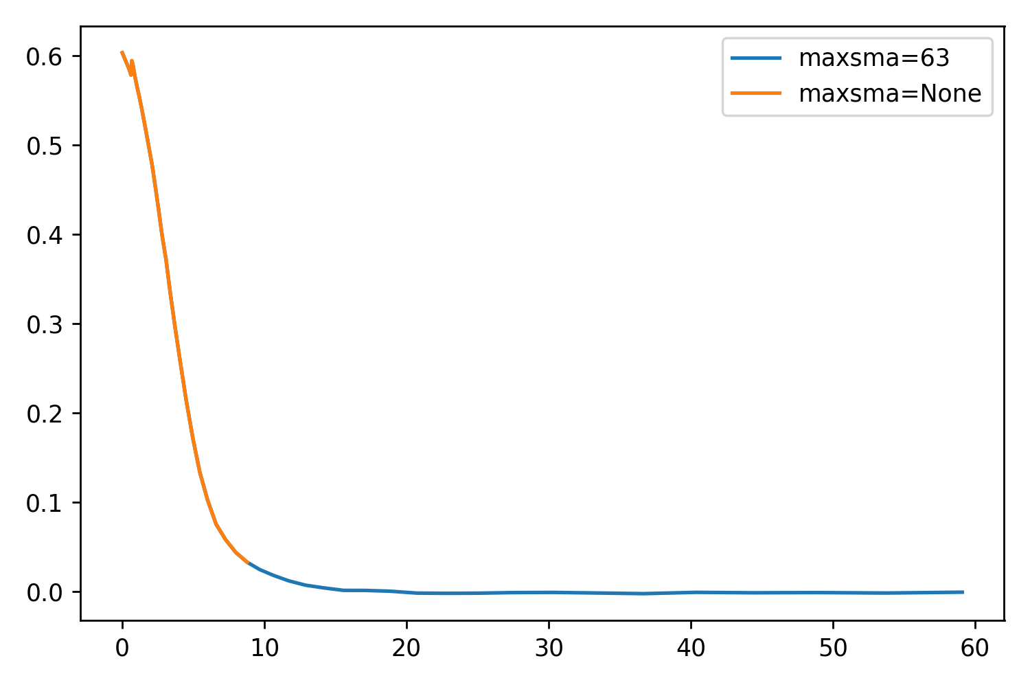
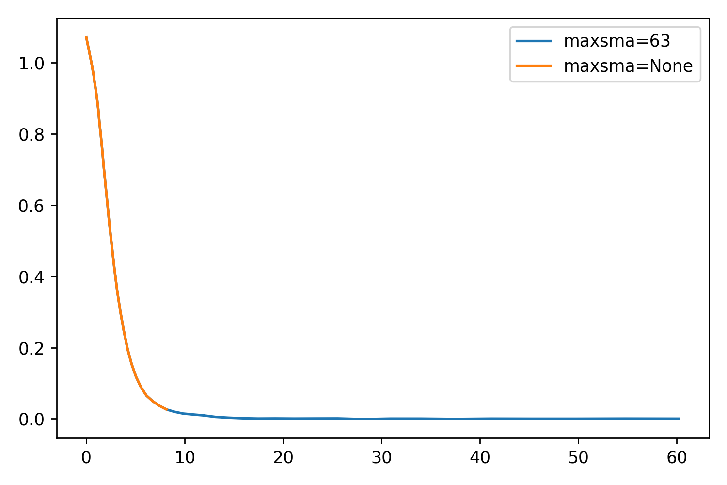
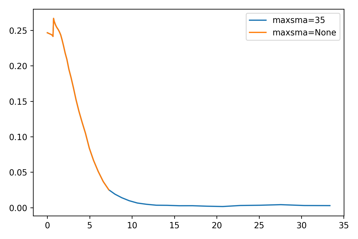
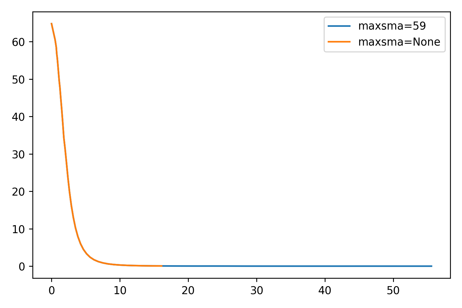
While testing maxgerr, I noticed that the sizes of the profiles were not increasing enough, even when setting the parameter very high. Returning to the other parameters, I noticed maxsma, which is defined as:
So by default, this parameter is set to None. If we set it to whatever value we like (say, the largest distance horizontally or vertically from the center to the cutout edge), we should be able to extend the profile even further. This will essentially be forcing the extraction as far as it can go.
I’ve included two things: A scatter plot showing just how well maxsma works, and a set of some example profiles. The one thing that is very optimistic about this parameter is that the profile is exactly the same up to reaching the stop criterion!
Here are the mass vs redshift and i-band magnitude vs redshift plots with their ranges readjusted.
Heat-maps
To get a better sense of what is going on in the above plots, we can plot bins of redshift and mass and see the ratio of successes to failures in each bin. In the total heat-map (2) I simply plot the number of objects in each bin. In the ratio heat-map (2) I divide the number of successes by the total.
Modelling
I fixed my modelling to be in line with the appropriate method. I generate a 2D model cutout, and refit both the observed cutout and the model cutout with the same parameters. I choose an arbitrary Sersic index of 0.5.
There are two noticeable things: The first is that the models tend to not extend further than the observed profiles. I believe this is because, based on the Sersic index, the profile (effectively) reaches 0 faster than the actual profile reaches the background.
Adjusting the Stop Criterion for Ellipse()
We also discussed the possibility of increasing the extent of the ellipse fitting method. The parameter in question, maxgerr, is defined in the documentation as : “The maximum acceptable relative error in the local radial intensity gradient. This is the main control for preventing ellipses to grow to regions of too low signal-to-noise ratio.” If we are fine with allowing the ellipses to grow, then there should be no issue with increasing this parameter.
To do some preliminary testing, I generated 50 profiles and corresponding cutouts that I knew were successfully fit. I then refit them using the original parameter setting (maxgerr = 0.5) and a higher setting (maxgerr = 2.0). I then plotted the maximum semimajor axis values (in pixels) of both on the same axis. As you can see, a higher parameter value results in profiles that tend to extend further.
However, there are a few below the line. Since we are interested in the larger profile, I propose that we generate both (upon finding a successful initial “guess” for the ellipse fitting). We then return the larger of the two. This will ensure the most information retrieved for each successful profile.
More Background Testing
Continuing on with testing the background algorithm on more cutouts, I used the same 50 profiles as used above and calculated the background value. I plot all of these on the same histogram as my last update to see where things fall. As you can see, the majority are well within the backgrounds generated from the manually selected empty regions. A few lie outside, but still they seem to be within 1 sigma of the median value. There is a very slight bias towards a brighter background, but as we talked about, being biased towards using slightly less of our profiles is the safer choice.
As we discussed, we want to effectively get a background estimate in our images. One suggestion was to find three empty areas in the image, obtain those cutouts, and redo the histograms. Below are three regions I manually selected at different areas of the image, along with the histogram of all pixel values in these regions. Surprisingly, the median values for these cutouts all lie below 0, as opposed to the cutout I was working with.
HSC Sky Subtraction
I was also taking a look at the DR2 release paper (Aihara et al., 2019, Section 4.1) to see their methodology of performing sky subtraction. There was some brief discussion about how the HSC images were sky-subtracted so I wanted to clarify things. Their method is rewritten to help with my own understanding below:
Generate 1024×1024 “super-pixels”, whose means are taken (ignoring pixels flagged as DETECTED)
A 6th order 2D – Chebyshev polynomial is fit to the super-pixels (I can only assume this is for smoothing and to help with interpolation in the next step)
Regular pixel positions are interpolated using Akima splines, which are piecewise polynomial functions that help to prevent outliers from affecting the data.
This generates a resultant background image, which is subtracted from the CCD image.
The 2D Chebyshev polynomial fitting would result in something akin to the figure below, which I found as a typical example of what these 2D functions look like. To help bolster my understanding I read section 18.4 of my Math Methods textbook that covers the 1D version.
They also generate a “sky frame” which involves the mean response of the instrument to the sky, related to the filter. Each filter has a characteristic spatial nature, seen in fig. 4. The subtraction is then a combination of fitting and subtracting both elements. Thus, the sky-subtraction is not uniform (I’m assuming this is what you meant by it being global!), and changes from band to band.
Their method got me thinking about ways I could estimate background in my own images. I think I have an idea of extending their methodology to my own work, although my method would be a lot simpler and “back-of-the-envelope”-esque. I outline a possible method below:
Generate a very aggressive mask (SNR = 0.5, Gaussian Width = 5, or some similarly aggressive mask parameters).
Take 10px by 10px “super-pixels” throughout the masked cutout, and take the median of all non-masked pixels.
For the background, we can reasonably assume that the minimum value we obtain out of all super-pixel medians will be the most faithful background value estimation.
An example of an aggressive mask is shown below. Before any extra coding is done, it can be seen visually that we should grab the lower background values in the left side of the image using this method.
I decided to test this method on few more cutouts. The cutout shown above results in a background estimate of BG=0.015. If I try a different object, I get a background estimate of BG=-0.004, which is both negative, and is right on the money when comparing to the mean of the three background estimates from the empty regions. This leads me to believe that the cutout I was working on just happens to be in a slightly brighter region. Perhaps!
The cutout that results in a near-perfect background estimationThe vertical red line is the estimate.
How Far the Profile is Extending
Below is an example profile, with the HLR plotted as the vertical line and the background estimation (old method with old masking parameters) plotted as the horizontal line. Units on the x axis are in pixels, units on the y axis is intensity. The termination value for this profile (and I have noticed that this appears consistent for most if not all of our profiles) is well above this background estimation, which we can take as already large. Is it possible that we can assume that the profiles we obtain are all valid so long as they lie above this (already larger than the true value) background estimate? It is my understanding that having a marginally larger BG estimate would be better for this sort of thing, as it would be safer in determining what can be used.
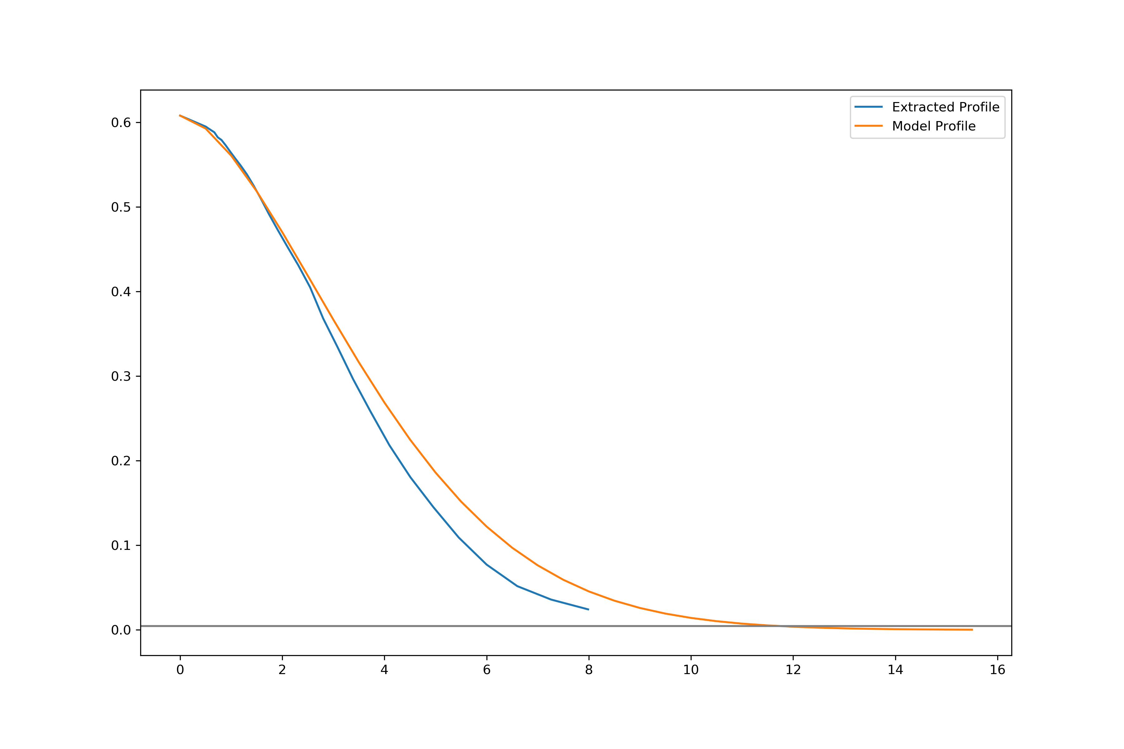
I also show below an example 1-D Sersic profile compared to an extracted profile. The parameters for the Sersic (which is normalized) are manually chosen to be a decent representation of the observed profile. The background value is shown exactly as above. I will also note that I allowed the model to extend twice as far as the extent of the observed profile.
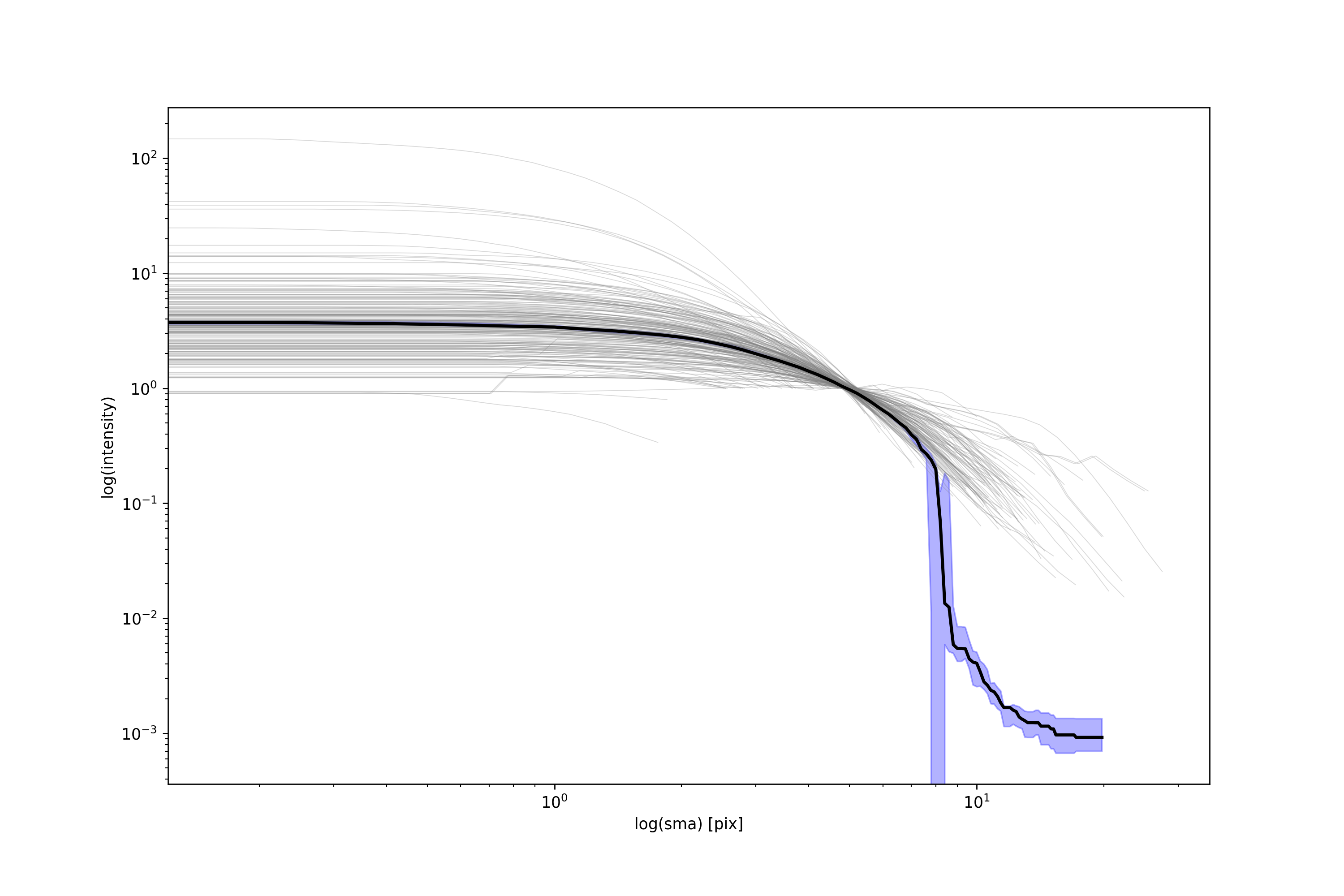
Medians Update
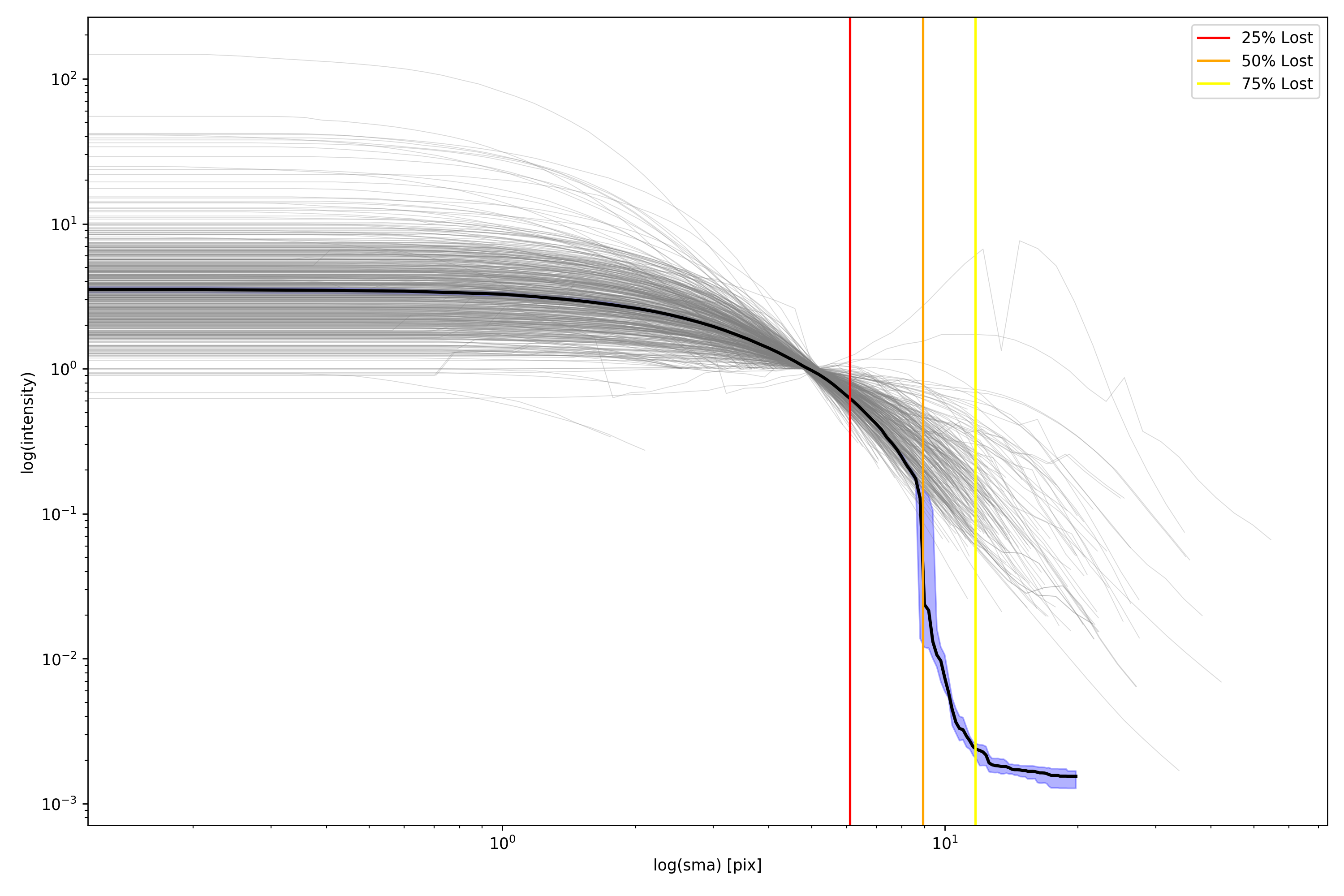
Here is a brief update to the medians! Below is a plot showing the plots and median for 500 galaxies. These galaxies are indeed normalized! I didn’t realize I had been doing that. Shown as 3 vertical lines are the locations where we lose 25%, 50%, and 75% of all our galaxies respectively. As expected, we start to see a drastic drop in the median once half our galaxies are lost. Currently, all of the interpolated profiles used in the median calculation extend to the same distance, so the number of galaxies in the median sampling remains the same throughout. The value used after we run out of valid data points is the extracted background value.
Finally, here are some plots showing M* vs z and i-band magnitude vs z!
At long last, Cedar is back up! This means I can finish up the processing jobs for the remaining few tracts in COSMOS I am also able to gather the good/bad IDs from the filespace.
Masking
Experiments with various parameters have proved fruitful. There are three parameters we can adjust to make an effect on the masking. These include the sigma value above the determined SNR ratio, the FWHM of the Gaussian filter kernel, and the number of pixels required for a collection of pixels to be considered as an object.
I experimented with various values in this parameter space, and have found that changing the number of pixels to be something higher than 5 is not necessarily a good idea. It does not have a tangible effect on the larger object, and it will only miss the smaller objects in the image. Below are plots showing the effect of various parameter settings on the masking. The left panel is the unmasked image, the middle panel is the segmentation map, and the right panel is the masked image.
Based on these results, I would say setting a sigma of 2.0 and a Gaussian size of 5.0 is the best option. It appears to strike a nice happy medium.
I also went and looked through the documentation on how photutils determines the “background” in detect_threshold(). Alas, there isn’t any real information on it. The method generates a pixel-wise threshold image, so the threshold changes in different regions of the image. It looks like it takes a median, and standard deviation from the input data (before masking) to determine a threshold.
Since I am able to get the IDs from Cedar, I also generated info plots for successful and unsuccessful fits. It is important to note that to save time in computation (and because my computer crashed when I tried to load everything into memory at once), only around 1/5 of all objects are included here. Below is the MvsZ plot for the i-band.
The paper has been updated with my first revision. This paper focuses mainly on the pipeline itself, going in depth into technical details and offering some information as to how it performs. If there is anything you want to suggest adding, please let me know!
Curious Issues with Medians
As I thought, the issue is not with my code. Below are plots of a single bin for 200 galaxies and 20 galaxies respectively, with the generated median and bootstrap error. As you can see, it holds up. I will look into if I am perhaps placing the medians in the wrong bin.
Quick and Dirty Modeling Tests
I have prepared some code that will use values retrieved from a galaxy via Ellipse to generate an output 2D Sersic Model. I select the Sersic index manually at the moment, but by the end of today I will fit the 1D profile with a sersic function and use the index from that fitting as my 2D model’s index.
Some interesting takeaways: Setting the hlr in the 2D Sersic model to twice the hlr value calculated from the profile (thus, the FWHM) results in a much more faithful profile. The position angle seems bang on, which is good! And the amplitude and its falloff outward from the centre (using a Sersic index of n=0.7) seems faithful to the data! You can also begin to see where the background cuts the observed object off as well, which is very interesting!
The first thing to mention is that all of Tract 9813 has been processed. This has netted us a grand total of 1.105 million objects. This works out (assuming an even distribution), to 160,000 unique objects. This is more than 10 times as much data as I had last year, and that is only for 1 tract! I am excited to see just how much we have for the entire field. Once Cedar is back up (starting tomorrow), I will finish fitting the remaining tracts. Then, I can figure out how many objects we have to work with in each band.
The current iteration of the matrix plot for COSMOS data is below. This matrix plot contains 5000 i-band images from one of the 9813 images. The x-axis is in units of Kpc and the y-axis is still in units of intensity. In order to convert to units of Surface Brightness, we will need a zero-point magnitude (which I’m not sure if I have or not!). There is also a lingering issue with the medians on the lowest row not plotting. I am still searching for the bug!
As Song Huang said, knowing what the background is for our images is a key factor in being able to push further into the outskirts for an object. To reiterate what he said, we effectively have two options. The first is to do what we are doing and simply create a cutoff at some arbitrary point where we say “after this point we aren’t going to trust the data we have”. The second is to better estimate the background and use that as a unique cutoff for each object.
Currently, I am estimating the background values for each of our objects. I am simply taking the mean value of all pixels that aren’t deemed as part of an object by the segmentation map. The masked pixels are set to this estimation. It’s a rough estimate, but does its job well for masking purposes.
Song also suggested to begin creating models with my output data. There is a BModel equivalent in the Photutils documentation; a method called build_ellipse_model(). There is an issue in that you require the original IsophoteList that the fitting creates, and not the table it generates. (The table is missing x0 and y0 parameters, along with gradients and harmonic information). I’ve created a pull request asking to include the gradient and x0,y0 parameters in the output table for the future. Here’s hoping the guys who maintain Photutils think it’s worth it!
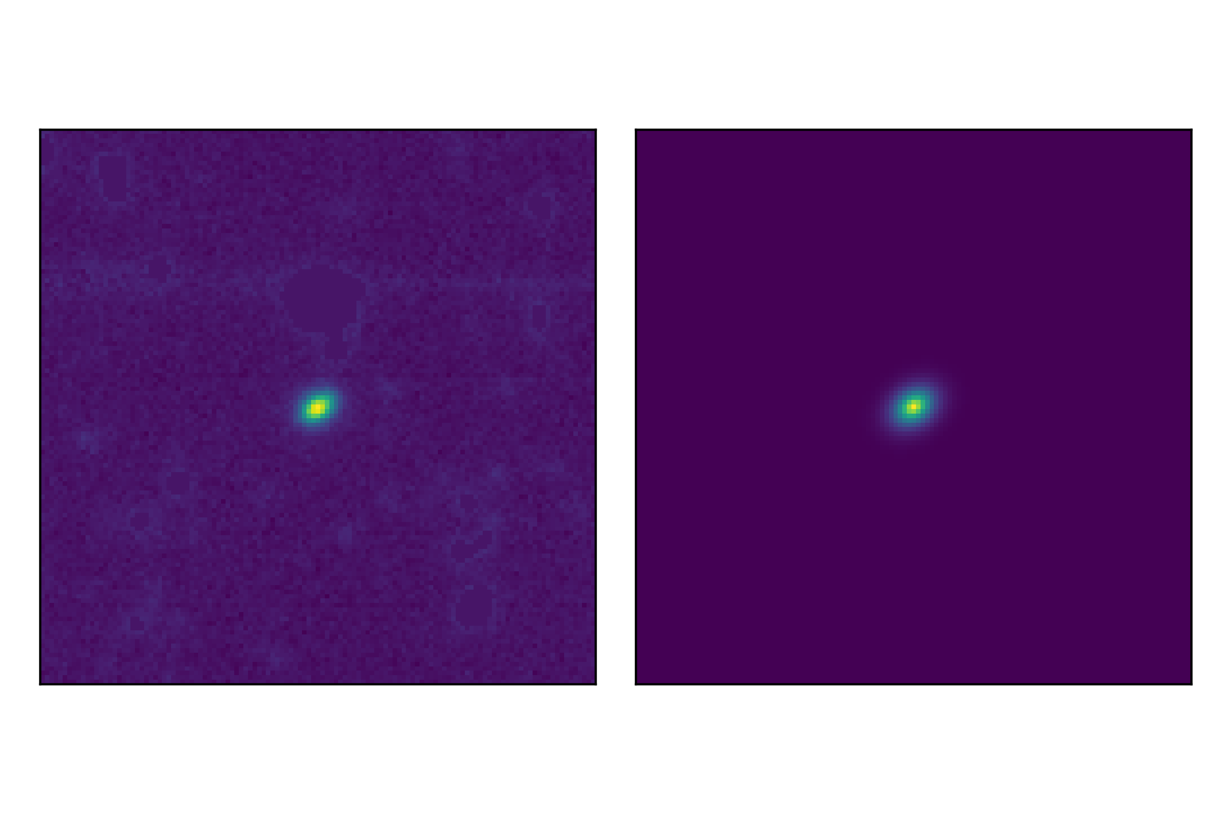
I have included below some examples of the models generated if I rerun my extraction method on some of the output cutouts. From left to right: The first image is the cutout data. The second image shows every 5th isophote overlaid on the cutout data. (Note: This is a new run of Ellipse() but it should return the exact same output as the pipeline does). The third image is the created model from the IsophoteList, and the 4th image is the residual (data – model).
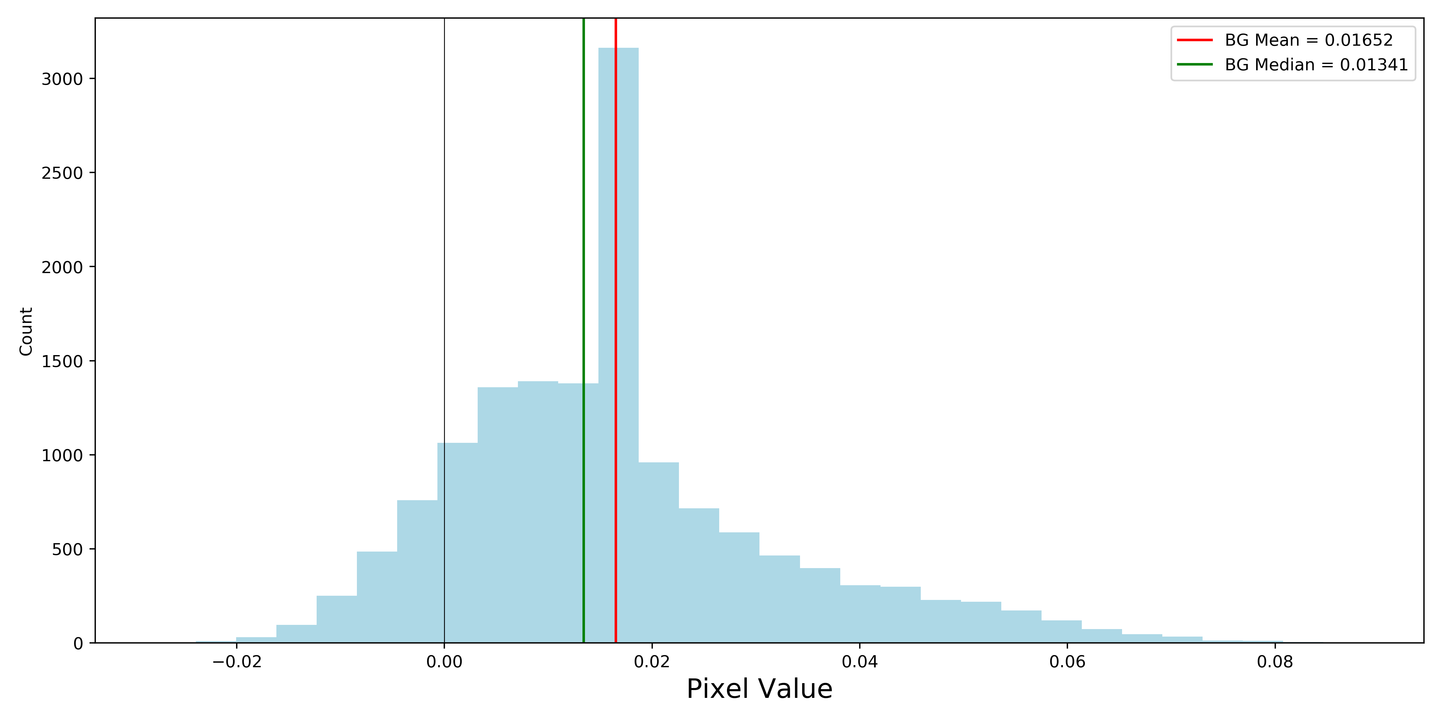
Below is a histogram of all background pixels for a heavily masked cutout. This is using the exact same SNR (3 sigma) to include pixels in objects as the already fit objects. The cutout in question is also included. The vertical lines correspond to the background mean value (what is currently being used as an estimate), and the median of background pixels. That spike in the histogram exists because of the masked pixels present in the image.
If we lower the SNR (down to 1 sigma), we get the following results. As you can see, the masking becomes slightly more aggressive. The distribution about the spike is a much more obvious standard distribution.
Given what we see in the second plot, could it be that the sky subtraction for this iteration of images is not strong enough? Since there is a standard distribution about a positive value, this is the conclusion that I can draw. Based on what you said Marcin, perfect sky subtraction would have this distribution about 0. Is it known whether or not these images have weak sky subtraction? Obviously this is for a single cutout, but I’m interested to see if this information is useful!
We are fully into production mode now! Out of the 10 tracts that exist in our sample, I have finished 4 of them and am currently fitting 9812 and 9814. The largest tract, 9813, is something I am going to try and tackle tomorrow. I plan to have all the processing done and my results moved off the cluster before Cedar goes into a 48 hour shutdown in 4 days.
One tract, 9571, returned 48320 galaxies! Assuming an even distribution across 5 bands (u and u* images only exist for 9813 and 10054), that’s over 9646 unique galaxies! Wow! I will also note this is for one of the smaller tracts. We should expect MUCH more for 9813 and 9812.
Finished F2 Field Processing
All possible profiles for galaxies and stars for the SHELS F2 field have been extracted. I wrote a utility script that compiles together 1 FITS file containing every unique object, so we don’t have a large set of individual files that we need to sort through. This will also be helpful once all our CLAUDS-HSC data is obtained.
I am currently working on a Jupyter notebook script that generates PSFs for our galaxies. This will save a third file, F2_PSFS.fits, which will have PSFs that can be ID matched. Configuring my Sersic fitting code to work with this data should be very simple!
Ivana, do you happen to have the data for the SHELS F1 field? I was thinking it might be worth it to also extract profiles for that field as well. Seeing as on AceNet, fitting the 20000 or so objects in F2 (duplicates included) took about 90 minutes, it wouldn’t be a large burden to gather those profiles to have in tandem with F2.
Pushing even further, the pipeline is now extremely easy to modify for any dataset you have, as it was rewritten with that in mind. Essentially, if you want me to extract profiles for basically anything that is available to you, I am more than willing to do so!
Paper Progress and an Interesting Find
I have also been working on filling out the MNRAS paper on the pipeline. While working last night, I figured it would be a good idea to work out the time per object, and that time whether it is succeeding or failing. I discovered after doing some tests that the time per failure and time per success differs per band! We do typically see a trend (except in the r band) of successful fits taking longer, and mean times hovering around 1 second per object. The reason why z, u and u* are not included is because the linear equations to solve for t_s and t_f didn’t return a valid answer (negative times for either success or failure).